Link to paper

The full paper is available here.

You can also find the paper on PapersWithCode here.

Abstract

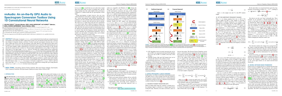
• Converting time domain waveforms to frequency domain spectrograms is typically done before model training.
• This approach has drawbacks, such as taking up a lot of hard disk space and needing to process audio clips again if another dataset is used.
• This paper proposes a neural network based toolbox, nnAudio, which leverages 1D convolutional neural networks to perform time domain to frequency domain conversion during feed-forward.
• nnAudio reduces the waveforms-to-spectrograms conversion time and further optimizes the existing CQT algorithm.

Paper Content

I. introduction

• Spectrograms have been used as input for neural network models since the 1980s
• Different types of spectrograms are tailored to different applications
• Despite advances in end-to-end learning, many recent publications still use spectrograms as input
• Applications include speech recognition, emotion detection, translation, enhancement, separation, conversion, tagging, cover detection, melody extraction, and transcription
• Training an end-to-end model on raw audio data takes longer and yields slightly better performance
• Finding the best spectrogram input requires trial and error and a lot of hard disk space
• Existing methods for time-frequency conversion are too slow for on-the-fly spectrogram extraction
• Tensorflow, Keras, and PyTorch have GPU-based spectrogram extraction methods
• None of the existing libraries support constant-Q transform
• nnAudio is a fast, differentiable, and trainable neural network-based audio processing framework
• nnAudio is built using PyTorch and includes extended functionalities such as calculating Mel spectrograms and constant-Q transforms

A. summary of key advantages

• Developed GPU-based audio processing framework
• Leverages power of neural networks
• End-to-end neural network training with on-the-fly time-frequency conversion layer
• Significantly faster processing speed than traditional audio processing
• Trainable Fourier, Mel and CQT kernels

Ii. signal processing: a quick overview

• Transformation methods used to convert signals from time domain to frequency domain
• Readers with signal processing background can skip this section

A. discrete fourier transform (dft)

• Audio signals are converted to digital signals before being stored.
• The Discrete Fourier Transform is used to convert the digital signal from the time domain to the frequency domain.
• The frequency domain output is in reverse order and only the first half of the frequency bins are extracted.
• The DFT is a split-sum of real and complex components.
• The frequency k in the DFT is given in terms of normalized frequency.

B. dft for arbitrary frequency ranges

• DFT is capable of resolving a finite number of distinct frequencies
• Frequency resolution can be improved by increasing window size
• Compromise between time and frequency resolution
• Applying DFT followed by inverse-DFT results in perfect reconstruction of original signal
• Modifying DFT to change frequencies of basis vectors
• Using log-frequency spectrogram to focus resolution in needed frequency range
• DFT and variable-resolution DFT used to calculate STFT using convolutional neural network

Iii. neural network-based framework

• Calculate STFT, Mel spectrogram, and CQT using 1D convolutional neural network
• Implement as library (nnAudio) in PyTorch 2
• Assumes basic understanding of convolutional neural networks
• Encodes audio processing knowledge into neurons of neural network
• STFT is fundamental operation for Mel spectrogram and CQT
• Multiply spectrogram by Mel filter bank kernel to convert to Mel spectrogram
• Compute CQT by beginning with STFT, followed by multiplication with CQT kernel

A. short-time fourier transform (stft)

• Short-time Fourier Transform (STFT) is an application of the DFT that cuts the signal into short windows before performing the transform
• Standard way to apply the DFT for audio analysis applications
• Cooley-tukey Fast Fourier Transform algorithm (FFT) computes the DFT in O(N log N ) operations
• O(N 2 ) DFT often outperforms the O(N log N ) FFT for small values of N when the underlying platform supports fast vector multiplication
• Neural network libraries typically include fast GPU-optimised convolution functions, which can be used to compute the canonical DFT quickly
• Discrete linear convolution of a kernel h with a signal x is defined as follows
• PyTorch defines a convolution function with a stride argument
• Can use convolution with stride to make fast GPU-based implementations of the STFT
• DFT is usually computed with a function that fades the samples at the edges of each window smoothly down to near zero
• Typical DFT window functions include Hann, Hamming, and Blackman types
• Can implement window smoothing efficiently by multiplying window function elementwise with the filter kernels before doing the convolution

B. mel spectrogram

• Mel frequency scale was proposed in 1937 to quantify pitch
• Several attempts to revise the Mel scale have been made
• There is not one “right” formula for the Mel scale
• Traditional frequency to Mel scale conversion is mentioned in O’Shaughnessy’s book
• Another form of the Mel scale is used in the Auditory Toolbox for MATLAB and librosa
• Mel filter banks are multiplied to each timestep of the STFT result to obtain a Mel spectrogram
• PyTorch 1D convolutional neural network is used to obtain the STFT results
• Mel filter banks are used to initialize the weights of a single-layer fully-connected neural network

C. constant-q transform 1) a quick overview of the constant-q transform (1992 version)

• Musical pitches have a logarithmic relationship
• Spectrograms need to use a logarithmic frequency scale
• Naive solution is to modify frequencies of DFT basis functions
• Orthogonality of basis is lost, leading to complicated energy relationship
• Gaps between frequency bins at upper end of spectrum
• Overlap between bins at lower end of spectrum
• Constant-Q transform (CQT) proposed by Brown in 1991
• CQT uses a logarithmic frequency scale
• CQT maintains constant frequency resolution by keeping constant Q value
• CQT and logarithmic frequency STFT have subtle differences
• CQT can be implemented with 1D convolutional neural network
• CQT kernels can be transformed to frequency domain
• CQT kernels can be huge if low frequency is used
• nnAudio API provides CQT function

3) downsampling

• Neural networks can be used to downsample input audio clips by a factor of two without aliasing.
• A low pass filter is required to filter out any frequencies above the downsampled Nyquist frequency.
• Finite impulse response filtering (FIR) is used to implement the low pass filter.
• The Window Method is used to design the low-pass FIR filter kernel.
• The CQT kernels are kept the same while the input audio is being downsampled recursively.

5) cqt with time domain kernels

• Brown and Puckette proposed an algorithm in 1992 that was more efficient in terms of memory
• Converting time domain CQT kernels to frequency domain kernels makes them more memory efficient
• With modern technology, memory is no longer an issue, so it is no longer necessary to convert the time domain CQT kernels to frequency domain kernels
• This modification improves the CQT computation speed

Iv. experimental results

• Analyzed speed and accuracy of proposed framework nnAudio
• Compared nnAudio to existing audio processing library librosa
• Compared STFT, Mel Spectrogram, and CQT implementations
• Compared to other existing GPU audio processing libraries
• Tested speed to process 1,770 audio files
• Tested correctness of resulting spectrograms
• Discussed CQT1992v2 and CQT2010v2 implementations

A. speed

1) setup

• Used MAPS dataset to benchmark nnAudio
• Discarded first 20,000 samples from each audio excerpt to remove silence
• Each audio excerpt kept same length (80,000 samples)
• Goal of speed test to convert array of waveforms to array of spectrograms
• Tested on 3 different machines
• Compared speed of nnAudio to librosa, Essentia, Kapre, Tensorflow, and Torchaudio
• Librosa with multi-process not used
• Caching disabled for librosa
• Only one GPU used for nnAudio
• nnAudio faster than librosa regardless of machine
• RTX 2080 Ti GPU performance similar to Tesla v100 GPU
• Extra time required to transfer kernels from RAM to GPU memory
• Initialization time influenced by kernel sizes of STFT, MelSpec, and CQT
• CQT2010 faster initialization time than CQT1992
• STFT, MelSpec, and CQT speeds shown in Figure 11
• CQT1992v2 and CQT2010v2 improve computation speed
• CQT2010v2 used for computers without GPU
• CQT1992v2 used when GPU available
• nnAudio faster than torchaudio and Kapre
• NVIDIA DALI not included as it does not calculate gradient for spectrograms

B. conversion output 1) setup

• Librosa is used as a benchmark to check the correctness of the implementation
• Four input signals are used to determine the model output correctness
• The chromatic piano scale is recorded with a piano instrument
• CQT1992v2 is faster and better quality than CQT2010 and CQT2010v2

2) results

• Results of accuracy test shown in Figures 12 and 13
• STFT and MelSpec results from librosa and nnAudio are very similar
• CQT output for nnAudio is smoother
• Comparison between CQT1992v2, CQT2010v2 and librosa’s CQT shown in Figure 14
• Aliasing due to downsampling is observable
• CQT1992v2 is fastest and best of all proposed GPU-based CQT implementations

V. example applications

• nnAudio can be used to explore different spectrograms as input for music transcription models.
• nnAudio allows STFT kernels to be trained/finetuned for better spectrograms.

A. exploring different input representations

• Music transcription can be done quickly with nnAudio
• nnAudio can explore different types of spectrograms as input for a neural network
• Four types of spectrograms are explored: linear frequency scale, logarithmic frequency scale, Mel spectrogram, and CQT
• Each spectrogram has different parameter settings to consider
• 34 different input representations are explored
• Transcription accuracy can be measured with mir_eval.multipitch.metrics()
• Input representation and its settings have a big influence on model performance
• nnAudio enables fast comparison of different representations
• nnAudio can be faster than pre-processed approach
• Time required for experimental phase can be drastically reduced with nnAudio

Index

• nnAudio allows us to integrate audio processing into a neural network model
• nnAudio allows us to store audio clips in the original waveform, without saving extra copies of the dataset for the spectrograms
• nnAudio is useful when the dataset is large and takes tens of hours to convert the data from waveforms to spectrograms

B. trainable transformation kernels

• STFT and MelSpec can be implemented with a 1D convolutional neural network
• Gradient descent can be used to finetune the kernels and filter banks
• STFT window size is set to 64 to make the task non-trivial
• 10,925 pure sine waves with different frequencies are generated to form the dataset
• 80% of the sine waves are used as the training set, 20% as the test set
• Two models are used to predict the frequency of the input signal: a fully connected network and a 2D convolutional neural network
• Trainable transformation layer results in a lower mean square error
• Trained Fourier kernels contain higher frequencies on top of the fundamental frequency
• Trainable Mel filter banks and CQT kernels allow a richer spectrogram to be obtained
• Higher-performing end-to-end model can be obtained with a trainable transformation layer

Vi. conclusion

• Presented a new framework for extracting spectrograms with neural networks
• Allows for dynamic training of kernels
• Implemented as GPU-based library, nnAudio
• Time domain to frequency domain transformation algorithms implemented in PyTorch
• GPU audio processing reduces time to convert waveforms to spectrograms
• Trainable kernels result in better model on frequency prediction task
• Proposed framework is first to support CQT
• CQT algorithm using time domain kernels performs faster than frequency domain kernels
• Computation time reduced drastically with nnAudio on real dataset, MusicNet