Link to paper
The full paper is available here.
You can also find the paper on PapersWithCode here.
Abstract
- DDPMs produce excellent samples
- DDPMs can achieve competitive log-likelihoods while maintaining high sample quality
- Learning variances of the reverse diffusion process allows sampling with fewer forward passes
- Precision and recall used to compare DDPMs and GANs
- Sample quality and likelihood of DDPMs scale smoothly with model capacity and training compute
Paper Content
Introduction
- Diffusion probabilistic models match data distribution by learning to reverse a gradual, multi-step noising process
- Denoising diffusion probabilistic models (DDPM) and score based generative models are equivalent
- DDPMs can produce high-quality images and audio
- DDPMs have yet to be shown to achieve loglikelihoods competitive with other likelihood-based models
- DDPMs can achieve loglikelihoods competitive with other likelihood-based models, even on high-diversity datasets
- DDPMs can generate audio using a small number of sampling steps
- DDPMs can be optimized with a hybrid learning objective
- DDPMs can sample in fewer steps with little change in sample quality
- DDPMs have higher recall than GANs for similar FID
- Performance of models increases with model size and training compute
Denoising diffusion probabilistic models
- DDPMs are formulated by Ho et al. (2020).
- DDPMs involve a fixed noising process q which adds diagonal Gaussian noise at each timestep.
- Sohl-Dickstein et al. (2015) provides a more general derivation.
Definitions
- A forward noising process is defined which adds Gaussian noise at each time step with variance βt.
- The latent xT is nearly an isotropic Gaussian distribution if T and βt are sufficiently large.
- A neural network is used to approximate the reverse distribution q(xt-1|xt).
- A variational lower bound is written as an equation which can be evaluated in closed form.
- The probability of pθ(x0|x1) landing in the correct bin is calculated.
- An arbitrary step of the noised latents can be sampled directly conditioned on the input x0.
Training in practice
- Objective in Equation 4 is a sum of independent terms
- Equation 9 provides an efficient way to sample from an arbitrary step of the forward noising process
- Ho et al. (2020) uniformly sample t for each image in each mini-batch
- Network can predict x 0 or noise to derive µ θ (x t , t)
- Reweighted loss function used to optimize L vlb
- Generative score matching used to explain better sample quality
- Variance fixed to σ 2 t I for best results
Improving the log-likelihood
- Ho et al. (2020) found that DDPMs can generate high-fidelity samples according to FID and Inception Score.
- DDPMs were unable to achieve competitive log-likelihoods with these models.
- Log-likelihood is a widely used metric in generative modeling and it is believed that optimizing log-likelihood forces generative models to capture all of the modes of the data distribution.
- Small improvements in log-likelihood can have a dramatic impact on sample quality and learnt feature representations.
- This section explores modifications to the algorithm that allow DDPMs to achieve better log-likelihoods on image datasets.
- Experiments were conducted on ImageNet 64 × 64 and CIFAR-10 datasets.
- The setup from Ho et al. (2020) achieved a log-likelihood of 3.99 (bits/dim) on ImageNet 64 × 64 after 200K training iterations.
- Increasing T from 1000 to 4000 improved log-likelihood to 3.77.
- The model parameterizes the variance as an interpolation between β t and βt in the log domain.
Improving the noise schedule
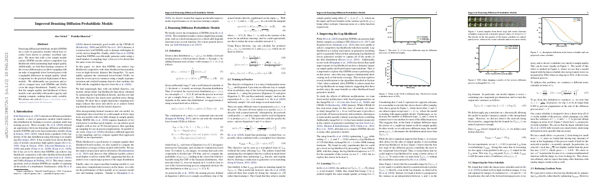
- Linear noise schedule works well for high resolution images, but not for 64x64 and 32x32
- End of forward noising process is too noisy and doesn’t contribute to sample quality
- Constructed a different noise schedule to address this problem
- Cosine schedule has linear drop-off in the middle of the process, while changing very little near the extremes
Reducing gradient noise
- Optimizing L vlb directly was expected to achieve the best log-likelihoods, but was difficult to optimize in practice.
- L hybrid achieved better log-likelihoods on the training set given the same amount of training time.
- The gradient of L vlb was much noisier than that of L hybrid.
- To reduce the variance of L vlb, importance sampling was employed.
- Optimizing L vlb with importance sampling achieved the best log-likelihoods.
Improving sampling speed
- 4000 diffusion steps are needed to produce a single sample on a modern GPU.
- Sampling can be done in a few seconds instead of minutes by reducing the steps used during sampling.
- Sampling noise schedule can be obtained from a given sequence of t values.
- Sampling steps can be reduced from T to K by using K evenly spaced real numbers between 1 and T.
- L hybrid model with learnt sigmas maintains high sample quality with 100 sampling steps.
Comparison to gans
- Likelihood is a good proxy for mode-coverage, but difficult to compare to GANs.
- Precision and recall used instead.
- Class-conditional models trained, class information injected through same pathway as timestep t.
- Two models trained, one BigGAN-deep model with 100M parameters.
- 50K samples generated for metrics, full training set used for FID.
Scaling model size
- Algorithmic changes can improve log-likelihood and FID without changing training compute
- Trend in modern machine learning is that larger models and more training time improve model performance
- Investigated how FID and NLL scale as a function of training compute
- Results suggest DDPMs improve in a predictable way as training compute increases
- FID scales according to a power law, NLL does not
Related work
- Song et al. (2020a) and Song et al. (2020b) propose fast sampling algorithms for models trained with the DDPM objective.
- Gao et al. (2020) develops a diffusion model with reverse diffusion steps modeled by an energy-based model.
- Our method allows fast sampling directly from the ancestral process, removing the need for extra hyperparameters.
Conclusion
- DDPMs can sample faster and achieve better log-likelihoods with little impact on sample quality
- Learning Σ θ using a parameterization and L hybrid objective improves likelihood
- Fewer steps are needed for sampling
- DDPMs match sample quality of GANs and have better mode coverage
- More training compute leads to better sample quality and log-likelihood
- DDPMs combine good log-likelihoods, high-quality samples, and fast sampling
- UNet model architecture used
- Attention layers use multi-head attention
- Model conditions on t using GroupNorm
- Model parameters and FLOPs estimated
- Smaller model used for CIFAR-10
- Dropout values {0.1, 0.2, 0.3} used
- Adam used for all experiments
- Batch size of 128 and learning rate of 10-4 used
- EMA rate of 0.9999 used
- 50K samples produced for most experiments
- 10K samples produced for unconditional ImageNet 64 × 64
- Training set used for CIFAR-10 and ImageNet
- 50K training samples used for LSUN
- L hybrid model outperforms DDIM with more than 50 diffusion steps
- L hybrid and L vlb combined to achieve FID of 19.9 and NLL of 3.52 bits/dim
- Strided subset of timesteps used to improve log-likelihood
- NLL not calculated for DDIM
- Overfitting observed on CIFAR-10 and ImageNet 64 × 64
- EMA hyperparameter of 0.9999 and 0.99995 worked best
- Dropout of 0.1 and 0.3 used
- Cosine schedule easier to optimize and overfit
- Two models trained on class conditional ImageNet 256 × 256
- VQ-VAE-2 used for comparison
- Diffusion models obtain best FIDs for likelihood-based model