Link to paper

The full paper is available here.

You can also find the paper on PapersWithCode here.

Abstract

• Developed a deep learning model to create a high-resolution canopy height map of the “Landes de Gascogne” forest in France.
• Model uses multi-band images from Sentinel-1 and Sentinel-2 with composite time averages as input.
• Evaluation performed with external validation data from forest inventory plots and a stereo 3D reconstruction model.

Paper Content

Introduction

• Forest biomass is important for global carbon cycle
• High spatial resolution needed to capture difference in biomass
• Top canopy height can be a proxy for forest biomass estimation
• Forest inventories provide reliable information but not high-resolution maps
• Remote sensing data can provide accurate height estimations
• Airborne LiDAR and space-borne measurements have potential to map forest properties
• GEDI LiDAR mission provides accurate point-wise observations
• Sentinel-1 and Sentinel-2 provide measurements at 10 m resolution
• Global and local maps of forest biomass and height have been developed
• Machine learning and deep learning have been used for forest parameter estimations
• CNNs have increased accuracy for image interpretation tasks
• CNNs have been used for tree height mapping

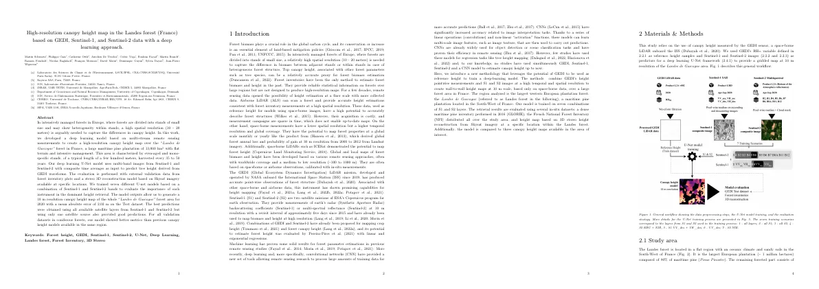
Materials & methods

• Used GEDI sensor to measure canopy height
• Used Sentinel-1 and Sentinel-2 images as predictors for a deep learning U-Net framework
• Produced a gridded map of the Landes de Gascogne area at 10 m resolution

Study area

• Landes forest is located in South-West France
• Comprised of 90% maritime pine and 10% broadleaved forests
• Intensively managed with thinning every 5-10 years and clear-cuts every 35-50 years
• Understory vegetation includes woody shrubs and perennial herbaceous plants
• GEDI data used to model continuous height map at 10 m resolution
• GEDI data acquired from ISS between 51.6° South and 51.6° North
• GEDI L2A product provides RH metrics representing height relative to ground
• RH 95 used as proxy for height
• 526,449 GEDI footprints downloaded from NASA’s EarthDataSearch
• Filtering criteria applied to remove unusable waveforms
• Study area divided into 117 tiles of 100 km²
• 91 Train tiles, 15 Validation tiles, and 11 Test tiles
• Uneven temporal and spatial distribution of data
• GEDI footprints in Test and Validation tiles removed if tree cover has null value in Copernicus tree cover density map
• Height repartition of data in Train, Validation, and Test datasets

Sentinel-1

• Sentinel-1 is a C-band Synthetic Aperture Radar mission with two satellites
• 280 images were selected over a five-month period in 2020
• Images were preprocessed with the Sentinel-1 toolbox in Google Earth Engine
• Backscattering coefficients (dB) measure the backscattered microwave radiations
• Per-pixel median of the images was calculated to create a single composite image of 4 layers
• Values were restrained to -30 dB to 0 dB and scaled to a 0 to 1 interval

Sentinel-2

• Sentinel-2 mission is part of ESA’s Copernicus program
• Two satellites, Sentinel-2A and Sentinel-2B, launched in 2015 and 2017
• Provides multispectral images of Earth surface reflectance with a low revisit interval of ~5 days
• L2A product used provides bottom of atmosphere reflectance
• 13 spectral bands ranging from 10m to 60m resolution in visible, NIR, and SWIR
• 172 images selected from Google Earth Engine with less than 50% clouds
• Cloud mask applied and single composite image created by taking per-pixel median value
• 10 spectral bands kept and resampled to 10m
• DN values clipped in 0-5000 interval and divided by 5000 to create range of 0-1
• Resulting composite image exempt from cloudy areas

Evaluation datasets

• Compared height predictions to 3 datasets of different spatial scales
• Compared predictions to canopy height maps from previous studies

Forest inventory data

• Good correlation between predicted height and GLORIE dataset (R² coefficient of 0.93)
• Higher prediction bias for heights from 0 to 10 m
• Good correlation between predicted height and IFN dataset (R² = 0.71)
• Higher correlation and better error metrics for coniferous forests (R² = 0.79, RMSE = 3.09 m)
• Lower correlation and poorer error metrics for broadleaved forests (R² = 0.38, RMSE = 5.74 m)

Stereo 3d reconstruction from skysat imagery

• Skysat is a constellation of satellites providing high-resolution imagery
• Geolocation accuracy is 3.4 m
• Stereo 3D height reconstruction technique used to reconstruct 3D objects
• Digital surface model created from point-cloud 3D reconstruction
• Cloth simulation algorithm used to select ground points
• Laplace interpolation used to create a canopy height model
• Canopy height model compared to model outputs

Canopy height maps from previous studies

• Compared model predictions to 3 canopy height maps from independent studies
• Maps from Potapov et al. (2021) and Lang et al., (2022a) used GEDI
• Reference height measurements based on small local forest inventory of maritime pine only

Methodology

U-net model description

• Pixel-wise regression is the process of attributing a value to each pixel in an image.
• U-Net model adapted from Milesi (2022) is a fully convolutional network (FCN) that outperforms previous models in speed and accuracy.
• U-Net model has a contracting path and an expansive path which gives it its “U” shape.
• The model has 18 convolutional layers and ~17 Million trainable weights.

Training process

• Objective of training process was to adjust weights of FCN model to output canopy height map from multi-channel image
• 91 Train tiles randomly selected, weighted by number of GEDI footprints
• 2560x2560 m subset randomly selected from tile with at least one GEDI footprint
• 256x256 pixels image composed of S1 and S2 layers used as input of U-Net
• GEDI RH 95 values rasterized on 10 m grid aligned with S1 and S2
• FCN model output compared to reference height from rasterized GEDI data with MAE loss
• Gradient of loss calculated with respect to model weights and weights adjusted accordingly
• Training process done on Amazon AWS cloud platform with Pytorch library

Training scenarios

• 7 training scenarios were designed based on combinations of spectral and polarization layers
• The first FCN model was trained on all layers from S2 and S1
• The second and third FCN models were based on one source of data only (S2 or S1)
• The other FCN models were trained on subsets of S2 and S1

Used metrics

• Evaluated FCN model using MAE, RMSE, ME, and R²
• Decomposed MSE into SB, SDSD, and LCS to get more info on source of errors

Results

Canopy height model

• FCN model was trained using all Sentinel-1 and Sentinel-2 layers
• Scenario 1 provided best prediction results
• FCN model is able to predict a continuous canopy height map
• FCN model is able to retrieve high height differences between forest from non-forest areas
• Most errors are below 5 m except in areas close to forest borders

Gedi test set evaluation

• FCN model compared to RH 95 values for Test dataset
• Obtained MAE of 2.02 m, RMSE of 2.98 m, and R² of 0.73

Evaluation with independent datasets

Figure 9. comparison between the predicted height from the fcn model (scenario 1) for the year 2020 with the forest inventory dominant height from the glorie project (measurements made in 2016) (a), and with french national forest inventory (nfi, measurements made over 2017-2020) (b). for both graphs, the dotted line represents the x=y axis. the predicted height corresponds to the mean height of the pixels within the forest plot area. the french nfi (b) dataset is colored by year of sample and separated into broadleaved and coniferous forests. red circles indicate plots that are not considered in the calculation of the error metrics because of forest clear-cuts between the date of the forest inventories and the date of the s1 and s2 images.

3d reconstruction from stereo satellite acquisition

• FCN model follows same pattern as 3D CHM
• Good correlation between 3D CHM and FCN predictions
• 3D reconstruction has sharper delimitations between forest units
• FCN model tends to smooth transitions between forest units

Influence of sentinel-1 and sentinel-2 bands on height predictions

• Results from best training scenario (Scenario 1) show lower RMSE values when compared to other datasets
• Scenarios including only Sentinel-2 bands have lower performances
• Scenarios 6 and 7 lead to larger errors for all validation datasets
• SB is higher when FCN model is compared to forest inventory datasets
• LCS is dominant term of error for most validation datasets
• Correlation is better when compared to 3D Skysat height reconstruction model

Comparison with other canopy height maps

• FCN model was compared to three different canopy height maps (L22, P21, M19)
• FCN model and L22 predicted higher homogeneity within forest stands
• P21 and M19 showed higher variability between adjacent pixels
• FCN model produced more plausible outputs with clearer delimitations between forest stands of different heights
• FCN model had better error metrics than the other models except for broadleaved forests
• L22 had better performances over broadleaved forests
• FCN model had a lower bias than the other models
• L22 had a high bias but still had a good correlation with datasets
• All models had better performances on the Skysat 3D reconstruction
• P21 predicted most coniferous forests at ~ 15 m, most broadleaved forests at ~ 22 m and most other pixels at ~ 5 m
• L22 had a higher correlation than the FCN model but tended to predict higher heights
• M19 had a lower correlation but with almost no bias
• P21 showed a saturation effect for coniferous forests at around 15 m

Discussion

 smoothness

• Smoothing effect observed in predictions compared to 3D reconstruction from stereo Skysat images
• Each pixel of the FCN canopy height map is the result of multiple convolutions involving the surrounding pixels
• Pixels close to forest borders have neighbor pixels from forest and bare soil which could lead to average height prediction, creating smoothness between landscapes units
• 10 m x 10 m S1 and S2 pixels on forest borders contain average information from both forest and non-forest areas and are also “smoothed”
• FCN model tends to predict average values at forest borders to avoid making high errors during the training process due to GEDI location uncertainty

 bare soil

• Bare soil is retrieved with a height of ~2.25 m
• Low non-forest heights are overestimated
• Overestimation of lower heights is related to RH 95 effect
• Tree growth effect accentuates this phenomenon

 underestimation at high forest heights

• Model underestimates heights above 20 m
• Phenomenon is common in most studies
• Imbalanced distribution of reference height labels
• Better performance over coniferous forests
• More S1 & S2 layers improves prediction
• S2 spectral bands with 10 m resolution are necessary
• Combination of two S1 layers leads to better results
• FCN model shows improved performance compared to other models
• Deep learning techniques are “spatially aware”

 on the use of gedi

• GEDI mission provides high precision LiDAR waveforms
• GEDI has potential for forest parameter estimation
• GEDI has difficulty retrieving canopy height in complex forest structures
• GEDI laser beams may not penetrate deep enough to reach ground, leading to height underestimation
• GEDI footprint location uncertainty can lead to large errors
• MAE improved from 2.43 m to 2.02 m when using more recent version of GEDI
• FCN model outputs show clearer patterns and transitions with more recent version of GEDI

 influence of the number of training samples

• GEDI footprints are unevenly distributed globally
• Fewer waveforms available in some regions
• Assessed how this affects reproducibility of proposed method
• Trained 3 additional models with 10%, 1%, and 0.1% of original train dataset
• Model with 10% of original train dataset still leads to good results
• Output map looks a little noisier with 1% of original sample size
• Results stress importance of having large training datasets
• Model still has good performances with 10% of original train dataset size

Concluding remarks

• Study highlights potential of deep learning models to map forest height continuously at high resolution
• GEDI LiDAR data and continuous images from Sentinel-1 SAR and Sentinel-2 multispectral imager used
• GEDI data produces good estimation of forest height when integrated into deep learning prediction model
• FCN model able to retrieve forest height at 10 m resolution with MAE of 2.02 m
• High correlation with independent height measurement sources
• Improved results compared to other existing canopy height models
• Methodology applied to another French “sylvoecoregion” called Sologne with MAE of 2.62 m
• Canopy height map could be used to monitor tree height with yearly time frequency
• Strong relationship between canopy height and canopy biomass
• Original model (MAE = 2.02 m) performs slightly better than modified model (MAE = 2.19 m)
• Original 10 m model able to retrieve heterogeneous canopy cover
• Model input data and model predictions on four different areas in Test tiles
• Predictions relatively well scattered around y=x axis
• Almost no bias for height values between 5 m and 20 m
• Comparison of GEDI height and predicted values from FCN prediction model
• Map of forest predicted canopy height over Landes forest for 2020
• Comparison of FCN prediction model for Scenario 1 (2020) and 3D canopy height model (3D CHM) based on Skysat imagery (2021)
• Error metrics on four evaluation datasets for 7 training scenarios
• Comparison of FCN model with three independent canopy height models
• Evaluation of FCN model against data from GLORIE forest inventory, French NFI, and 3D height reconstruction from Skysat imagery
• Evolution of MAE on Test dataset for 4 different FCN models trained with different sizes of Train dataset