Link to paper

The full paper is available here.

You can also find the paper on PapersWithCode here.

Abstract

• Interpretability methods can produce plausible explanations, but have also seen failure cases.
• It is unclear how to use these methods and choose between them.
• Feature attribution methods can fail to improve on random guessing for inferring model behaviour.
• End-tasks should be defined and a simple approach of repeated model evaluations can outperform complex feature attribution methods.

Paper Content

Introduction

• Feature attribution methods are used to answer local counterfactual questions about machine learning models
• These methods fall into two categories: first-order approximations and methods that incorporate how the model behaves on a baseline distribution
• The failure modes of local, first-order methods are well understood
• Common conceptions are that gradients never work and complete and linear methods are more reliable
• We show that complete and linear methods are often less reliable than simpler methods at answering local counterfactual questions
• Positive feature attribution does not imply that increasing the feature will increase the model output
• Zero feature attribution does not imply that the model output is insensitive to changes in the feature
• These methods can also fail to infer counterfactual model behaviour on average over models
• Brute-force approach of querying the model many times can be used to solve these questions

Problem framework

• Counterfactual model behaviour is a type of model behaviour that is the center of the study
• It is related to common tasks such as recourse and spurious feature detection
• It is defined as a model’s dependence on a feature j near an example x
• It is formulated as a hypothesis testing problem
• It is used to measure the performance of feature attribution methods
• It is related to tasks such as algorithmic recourse and distinguishing between models that globally ignore a feature and those that are sensitive to local perturbations

Framing the problem: hypothesis testing

• A natural framework to formalize the task of inferring counterfactual model behaviour is statistical hypothesis testing.
• The user’s goal is to determine whether the model has certain behaviour (null hypothesis) or different, plausible model behaviour (alternate hypothesis).
• The null and alternate hypotheses should encode necessary questions that must be answered to succeed at the task.
• After collecting information about the model, the user will conduct a hypothesis test and either reject or fail to reject the null hypothesis.
• The user may rely on external randomness to decide whether to accept or reject the null hypothesis.
• Feature attribution methods take as input the model, an example to localize, and a baseline.
• The quality of a hypothesis test is determined by its specificity and sensitivity.
• This framework differs from other hypothesis testing, such as t-testing.

Notation

• For any integer i, [i] = {1, …, i} and e i is the ith standard basis vector
• For any set A, A c is its complement and ∅ is the empty set
• For any example x ∈ X, x j is the jth element/feature
• f (z) is evaluated where z ∈ R p is defined such that for some examples x, x ∈ X and feature j ∈ [p]
• For any matrix M, M j is the jth row of M
• Capital letters denote random variables, µ ∈ P(X) and f : with similar notation for variances, covariances, etc.
• µ j is the jth marginal distribution of µ

Impossibility theorems

• It is impossible to conclude that the user does better than random guessing at inferring counterfactual model behaviour using common feature attribution methods without strong additional assumptions.
• Two common end-tasks are also impossible to conclude that the user does better than random guessing for.
• Even for very simple models, these feature attribution methods provably still incorrectly infer counterfactual model behaviour.
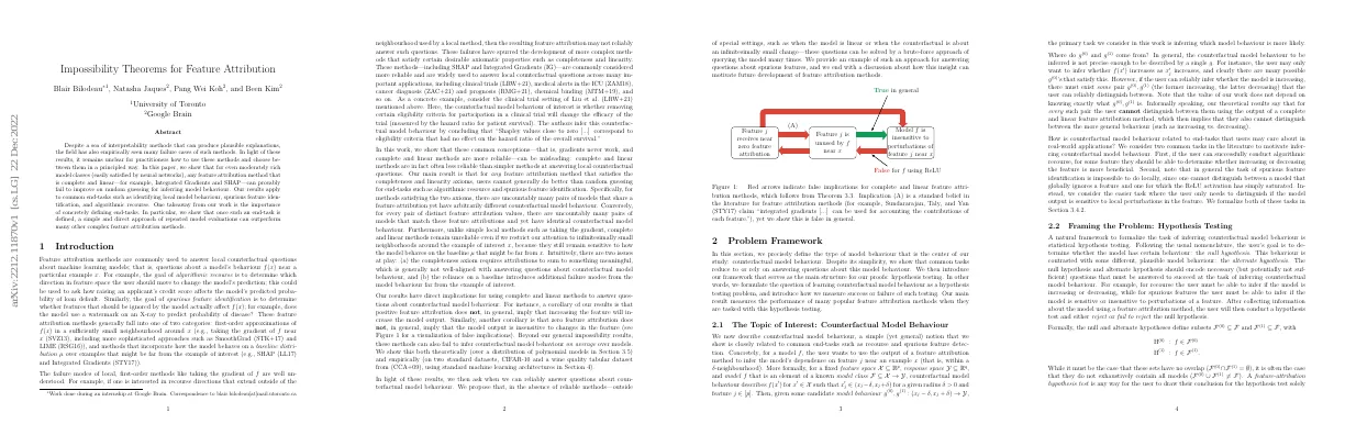
• Two commonly used properties of feature attribution methods are completeness and linearity.
• Two of the most common feature attribution methods, SHAP and Integrated Gradients, are complete and linear.
• Two mild assumptions about the features and the model class are required.
• The model class must be able to represent sufficiently many piecewise linear extensions of the local counterfactual model behaviour.
• The model class must include piecewise linear functions away from the region of interest.

Main result

• Theorem 3.3 states that for any counterfactual model behaviour, the best tradeoff between sensitivity and specificity that can be achieved by complete and linear feature attribution methods is no better than the tradeoff achieved by random guessing.
• Theorem 3.4 states that for any attribution φ ∈ R q , there exists a model f ∈ F such that for every complete and linear feature attribution method, Φ(f, µ, x) j = φ.
• Theorem 3.3 shows that without imposing additional assumptions on the underlying data or learning algorithm to significantly reduce the model complexity, the user cannot conclude that they have learned any information about the model.
• Proposition 3.5 states that for every ε > 0, x ∈ X , and j ∈ [p], there exists δ > 0 such that if then there exists h using Φ = Gradient such that for every µ ∈ P(X ) Spec Φ,µ,x (h) = Sens Φ,µ,x (h) = 1.
• Proposition 3.6 states that for every sufficiently small ε, δ > 0, x ∈ X , and j ∈ [p], if then for every feature-attribution hypothesis test h, complete and linear feature attribution method Φ, and µ ∈ P(X ) satisfying Assumption 1, Spec Φ,µ,x (h) ≤ 0.5 and Sens Φ,µ,x (h) ≤ 0.5.
• Proposition 3.7 defines recourse as a task of identifying whether a model output is locally sensitive to perturbations of a feature.
• Proposition 3.8 defines spurious features as a task of distinguishing whether a model is sensitive or insensitive to perturbations.
• Corollary 3.9 states that for any complete and linear feature attribution method Φ and feature-attribution hypothesis test h, the user cannot distinguish whether increasing or decreasing the feature is the correct direction to increase the model prediction, or whether the model prediction is sensitive to changes in the feature.
• Proposition 3.10 states that for the simple class of univariate models F = {x → ax n − x : a ∈ R} for some fixed n ≥ 2, on average over the models, for any complete and linear feature attribution method Φ and feature-attribution hypothesis test h, Spec Φ,µ,x (h) ≤ 0.5 and Sens Φ,µ,x (h) ≤ 0.5.

Experiments

• SHAP and IG do not provide enough information to accurately predict counterfactual model behaviour
• Results apply to neural networks trained with stochastic gradient descent on real datasets
• Experiments show SHAP and IG are close to random guessing for algorithmic recourse and spurious feature identification

Methods

• Estimate specificity and sensitivity of feature attribution method
• Conduct independent repetitions of experiment
• Sample new training and test data
• Train neural network with fixed architecture
• Compute multiple feature attribution methods
• Convert output of feature attribution method to hypothesis test
• Compare output of hypothesis test to ground-truth
• Use uniform distribution to compute ground-truth
• Hypothesis test based on positive/negative feature attribution
• Evaluate feature attribution method on tabular and image data
• Train convolutional neural network to reasonable accuracy

Results

• Experiments plot two outcomes: tradeoff of specificity and sensitivity, and accuracy of hypothesis test
• Tradeoff and accuracy are measured relative to best accuracy that can be achieved by random guessing
• For recourse task, both methods achieve same sensitivity/specificity trade-off and accuracy as random guessing
• For spurious feature task, same behaviour on wine quality dataset, but for convolutional neural networks on CIFAR-10, SHAP and IG achieve better sensitivity and specificity than random guessing
• This does not lead to overall improvement in accuracy
• Brute-force solving end-tasks via repeated model evaluations is guaranteed to work
• Theorem 5.1 shows that spurious feature identification can be solved without needing existing feature attribution methods
• Hypothesis test in Theorem 5.1 is designed to always succeed, but may be inefficient for more structured models
• Open problem: identify method that always succeeds at end-tasks of interest and is more efficient for problem structure of interest

Related literature

• Feature attribution methods can fail for algorithmic recourse near decision boundaries
• Feature attribution methods can fail to reliably infer counterfactual model behaviour
• Feature attribution methods can fail to match model behaviour in the exact local region of interest
• Various ways to formalize feature attribution have been proposed
• Counterexamples exist for common feature attribution methods
• Hypothesis testing can be used to formally compare feature attribution methods

Conclusion

• Feature attribution methods are currently used in high-stakes settings, but their performance is not well understood.
• This paper studied conditions under which feature attribution methods are unreliable.
• Using feature attribution as is currently prescribed does not improve on random guessing.
• To improve performance, more structure needs to be built into the methods.
• A brute-force method is guaranteed to work for some end-tasks, but it is computationally expensive.
• Accurately defining the end-task is crucial.
• Directly optimizing the task can provide straightforward answers.
• Interpretability goals are achievable, but new methods may be needed.
• SHAP and Integrated Gradients are both complete and linear.
• There is a weaker version of Integrated Gradients in the literature.
• For SHAP, there are two possible definitions in the literature.
• There is a proof technique for a multivariate version of SHAP and Integrated Gradients.
• There is a proof technique for a version of SHAP and Integrated Gradients with a single baseline example.
• There is a proof technique for a version of SHAP and Integrated Gradients with a baseline distribution.
• There is a proof technique for a version of SHAP and Integrated Gradients with a neighbourhood around a point.
• There is a proof technique for a version of SHAP and Integrated Gradients with a Gaussian CDF.
• There is a proof technique for a version of SHAP and Integrated Gradients with a query algorithm.