Link to paper

The full paper is available here.

You can also find the paper on PapersWithCode here.

Abstract

• Small training set sizes can be approximated by an infinite width neural network.
• After a critical sample size, finite-width networks become worse than infinite-width networks.
• Finite-size effects can become relevant for very small dataset sizes.
• Variance of the neural tangent kernel can explain the transition.
• Feature learning and ensemble averaging can push the transition to larger sample sizes.

Paper Content

Introduction

• Deep learning systems are achieving state of the art performance on a variety of tasks
• How generalization is controlled by network architecture, training procedure, and task structure is not fully understood
• Infinite-width networks yield a kernel method known as the neural tangent kernel
• Kernel methods are easier to analyze, allowing for accurate prediction of the generalization performance of wide networks
• Infinite-width networks can also operate in the meanfield regime
• Real networks have finite width, making analysis more difficult
• Unknown at what value of the training set size the effects of finite width become relevant
• Learning curve for the NN is well-captured by the learning curve for kernel regression
• Fluctuations in the final NTK over random initializations are suppressed at large width N and large feature learning strength
• P ∼ √ N transition and improvements due to feature learning through an alignment effect
• Variance contribution to generalization error can be reduced through ensemble averaging and feature learning

Problem setup and notation

• Supervised task with dataset D of size P
• Experiments focus on training networks to interpolate degree k polynomials on the sphere
• Generalization error scales as 1/P2
• Single output feed-forward NN with hidden width N
• Activations for an input x given by h
• Output of the network is fθ = h (L)
• Positively homogenous function (ReLU nonlinearity)
• Weights W ij ∼ N (0, 1)
• Scale of the output at initialization is O(σ L )
• Scale of the output is given by α = σ L
• Parameters trained with full-batch gradient descent on a mean squared error loss
• Generalization error approximates population risk

Empirical results

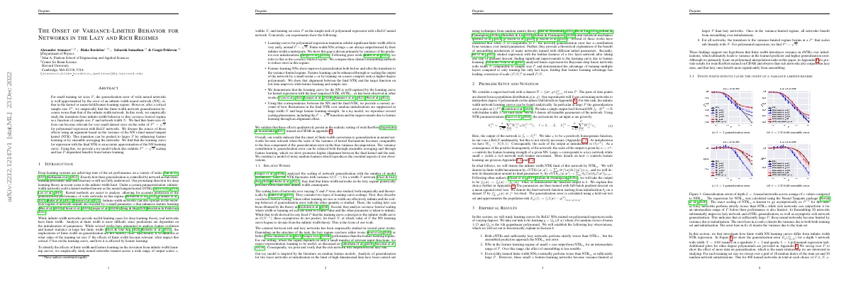
• Study learning curves for ReLU NNs trained on polynomial regression tasks
• Establish key observations
• NNs with small α can outperform NTK ∞ for an intermediate range of P
• Ensembling is less notable for small α
• Richly trained finite width NNs eventually perform worse than NTK ∞
• All networks benefit from ensembling in variance-limited regime
• Transition to variance-limited regime begins at P* that scales sub-linearly with N

Finite width effects cause the onset of a variance limited regime

• Finite width neural networks (NNs) and Neural Tangent Kernels (NTKs) have discrepancies that are explored in the paper.
• Ensemble averaging is used to calculate the error of the NNs.
• Phase plots are used to show the generalization, variance and kernel alignment of the NNs.
• Variance is lower for small α.
• Kernel alignment is related to good generalization.
• Most of the variance is due to initialization.

Final ntk variance leads to generalization plateau

• Variance over initialization can be interpreted as kernel variance in both the rich and lazy regimes
• All networks have same generalization error as kernel regression solutions with their final eNTKs
• Properties of eNTK f have been studied in prior works
• Final network generalization error matches generalization error of eNTK f
• Variance of final predictor related to corresponding infinite width network
• Finite size fluctuations of kernel at initialization have been studied
• Variance of kernel elements scales as 1/N
• Bias-variance decomposition holds for rich networks at small α

Feature learning delays variance limited transition

• Feature learning alters the onset of the variance limited regime.
• The onset of the variance limited regime is defined as the point where over half of the generalization error is due to variance over initializations.
• P 1/2 scales as √ N for this task.
• The delay of the variance limited transition is due to the kernel variance at initialization scaling as σ 2L /N.

Signal plus noise correlated feature model

• NN generalization error is approximated by kernel regression solution with eNTK f
• Analysis of generalization of kernel machines depending on network initialization θ 0
• Kernel generalization theory developed with statistical mechanics
• Attempt to derive approximate learning curves in terms of eNTK f’s signal and noise components
• Kernel interpolation problem solved by performing linear regression with features ψ(x, θ 0 )
• Averaging kernel directly and performing regression with this kernel exhibits largest reduction in generalization error

Toy models and approximate learning curves

• Characterize the test error associated with a Gaussian covariate model in a high dimensional limit
• Expected generalization error has a specific form
• Experiments show predictive accuracy of the theory
• Compute explicit learning curves for a simple toy model
• Replica calculation demonstrates that test error is self-averaging

Explaining feature learning benefits and error plateaus

• Kernels exhibit fluctuations over initialization with variance O(1/N)
• Small width networks enter the variance limited regime earlier and have higher error
• Altering the scale of the noise affects transition time and asymptotic error
• Transition occurs around P ∼ √ N
• Feature learning leads to improvements in the learning curve before and after onset of variance limits
• Enhancement of signal eigenvalue leads to lower bias and lower asymptotic variance

Conclusion

• Performed an empirical study on deep ReLU NNs learning a polynomial regression problem
• Performance worse than infinite width limit due to initialization variance
• Onset of variance limited regime can occur early with P 1/2 ∼ √ N
• Random-feature model used to explain and reproduce observed behavior
• Implications for choice of initialization scale, neural architecture, and number of networks in an ensemble
• Generated dataset by sampling x µ uniformly on unit sphere in R D
• Used JAX for neural network training
• MLPs of depth 2 and 3 used, no bias terms
• Trained with full batch gradient descent with learning rate η
• Swept over 15 values of P in logspace from size 30 to 10k, and 6 values of N in logspace from size 30 to 2150
• Swept over alpha values 0.1, 0.5, 1.0, 10.0, 20.0
• Saved generalization error, vector of ŷ predictions, initial and final parameters
• Applied same methodology of centering network and allowing α to control degree of laziness
• Binary classification task for CIFAR-10, subsampled 8 classes into 2
• Initial learning rate η 0 = 10 −3 , trained for 24,000 steps
• Swept α from 10 −3 to 10 0 and P from 2 9 to 2 15
• Ensembles of size 20, randomly sampled 5 training datasets of size P
• Symmetric decomposition of generalization error in terms of variance due to initialization and variance due to dataset
• Bagged predictor does not have substantially lower generalization error
• Most of variance driving higher generalization error is due to variance over initializations
• Fraction of E g that arises from variance due to initialization, variance over datasets, and total variance for width 1000
• Leading order terms have mean zero around their infinite-width limit
• Ensemble averages of feature learning networks have same generalization as infinite-width mean field solutions
• Change in output scales as O(1), change in features scales as (α √ N ) −1
• Used kernel alignment metric for diagonally dominant kernels