Link to paper
The full paper is available here.
You can also find the paper on PapersWithCode here.
Abstract
- Counterfactual explanations are important for detecting bias and improving explainability of data-driven classification models.
- Counterfactual explanations are minimal perturbed data points that cause the model’s decision to change.
- Existing methods can only provide one CE, which may not be achievable for the user.
- This work provides an iterative method to calculate robust CEs that remain valid even after features are slightly perturbed.
- The method provides a region of CEs, allowing the user to choose a suitable recourse to obtain a desired outcome.
- The method is applicable to logistic regression, decision trees, random forests, and neural networks.
- Experiments show the method can generate globally optimal robust CEs for a variety of data sets and classification models.
Paper Content
Introduction
- Counterfactual explanations are a way to explain decisions made by black-box machine learning models.
- The aim is to find a counterfactual feature combination that will lead to a flipped model prediction.
- User agency is provided by these methods, but the generated CEs are exact point solutions that may be difficult to implement in practice.
- Prior work suggests generating several CEs to increase the likelihood of generating an attainable solution.
- Robustness in CEs has different meanings, including robustness to input perturbations, model changes, hyperparameter selection, or recourse.
- Our work addresses robustness to recourse by utilizing a robust optimization approach to generate regions of CEs.
- Our method generates a set of CEs such that every solution in this set is a valid CE.
- Our approach is able to provide deterministic robustness guarantees for the CEs generated.
- We propose an iterative algorithm that effectively finds optimal robust CEs for decision trees, ensembles of trees, and neural networks.
- We prove convergence of the algorithm for the prementioned models.
- We analyze the performance of the algorithm on several datasets.
- We release an open-source software called RCE to make the proposed algorithm easily accessible.
Robust counterfactual explanations
- Binary classification problems involve assigning a value between 0 and 1 to each data point in a data space.
- A point is predicted to be in class +1 if the value is greater than or equal to a given threshold parameter, and class -1 otherwise.
- The robust CE problem is defined as finding a point as close as possible to a factual instance such that all perturbations of the point are classified as +1.
- Uncertainty sets are of the type where and duality is used to solve the optimization problem.
Adversarial robust approach
- Propose to solve a model with an iterative method known as the adversarial approach
- Consider a relaxed version of the model with a finite subset of scenarios
- Optimal value of the relaxed version is a lower bound of the original problem
- Solution of the relaxed version may not be feasible for the original problem
- Find a new scenario to cut off the solution of the relaxed version
- Maximize the constraint violation in the objective function
- If optimal value is positive, add the scenario to the set and calculate a solution
- Iterate until no violating scenario can be found
- Use accuracy parameter to guarantee convergence
- Handle the case of decision trees and tree ensembles
Linear models
- Algorithm 1 can be used to solve linear models.
- There is an easier and more efficient way to solve model (3)-(4).
- Validity constraint (4) can be formulated as β ∈ R n and β 0 ∈ R.
- These constraints can be reformulated as (7) and (8).
- (8) is linear in x regardless of S.
Decision trees
- Decision trees partition observations into distinct leaves through a series of feature splits
- Each leaf has been assigned a weight
- A Lipschitz continuous function is used to achieve convergence of the algorithm
- The classifier is a piecewise constant function
- The function is Lipschitz continuous except on the leaf boundaries
- Two formulations are derived for the tree model
- An alternative approach is proposed to find a CE which is robust only regarding to one leaf of the tree
- Iterating over all possible leaves is suggested to solve the resulting MP
- Auxiliary binary variables can be used to model the entire decision tree
Tree ensembles
- Random Forest (RF) and Gradient Boosting Machines (GBM) are tree ensembles
- Each base learner is a decision tree
- We add constraints to the master problem for each base learner
- We replace constraint (12) with a weight of leaf i in base learner k
- Random Forest is equivalent to a decision tree
- Convergence analysis from Section 2.3 applies to ensemble case
Neural networks
- Neural networks with ReLU activation functions are Lipschitz continuous and belong to the MIP-representable class of ML models.
- The ReLU operator of a neuron in layer l is given by a coefficient vector, bias value, and output of neuron j of layer l-1.
- The input of the neural network can be a data point perturbed by a scenario.
Experiments
- Aim to illustrate effectiveness of method by conducting empirical experiments
- Experiments run on computer with Apple M1 Pro processor and 16 GB RAM
- Open-source implementation available at GitHub
- First approach generating region of CEs for range of different models
- Experiments on 3 datasets: BAN-KNOTE AUTHENTICATION, DIABETES, and IONOSPHERE
- Features scaled to be between 0 and 1
- Algorithm used ∞-norm as uncertainty set with radius of 0.01 and 0.05
- Time limit of 1000 seconds
- Results in Table 1
Discussion and future work
- Proposed robust optimization approach for generating regions of CEs for logistic regression, tree-based models, and neural networks
- Theoretically converges and supported through empirical study
- Generates explanations efficiently on a variety of datasets and ML models
- Scales well with the number of features
- Main computational challenge is solving the master problem
- Future work includes speeding up calculations, evaluating user perception, and implementing categorical and immutable features
A. lipschitz continuity
- Proof of Lemma 2.3 is shown by considering three cases
- Lemma 2.3 states that h is Lipschitz continuous with Lipschitz constant L
- Neural network constructed with ReLU activation functions can be written as a composition of linear and component-as well as piece-wise linear functions
- Composition of two Lipschitz continuous functions is Lipschitz continuous with Lipschitz constant L h L g
- Master problem (MP) and adversarial problem (AP) are formulated
- Results on three datasets are reported in Table 2
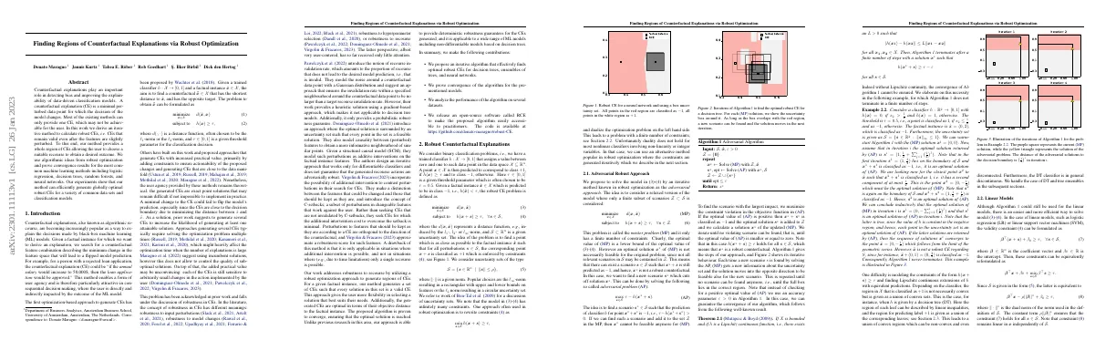
- Figures 2, 3, 4, and 5 illustrate iterations of Algorithm 1, slack values, and generation of robust CEs