Link to paper

The full paper is available here.

You can also find the paper on PapersWithCode here.

Abstract

• Cross-entropy loss improves with model size and training compute following a power law
• Intrinsic performance is a monotonic function of the return defined as the minimum compute required to achieve the given return
• Intrinsic performance scales as a power law in model size and environment interactions
• Optimal model size scales as a power law in the training compute budget
• Varying the “horizon length” of the task mostly changes the coefficient but not the exponent of this relationship

Paper Content

Introduction

• Recent studies have found relationships between neural network performance and model size/training compute to be governed by smooth power laws
• Studies have focused on generative modeling with cross-entropy loss
• This paper seeks to extend these results to reinforcement learning, which generally has no cross-entropy loss
• Introduces intrinsic performance, which is defined to be equal to training compute on the compute-efficient frontier
• Studies relationships between performance, model size and environment interactions across a range of environments

Intrinsic performance

• Cross-entropy test loss scales smoothly with training compute in generative modeling
• Mean episode return in reinforcement learning does not necessarily scale smoothly
• Intrinsic performance is a metric that behaves like test loss and scales as a power law with compute
• Intrinsic performance is the minimum compute required to train a model of any size to reach the same return

The power law for intrinsic performance

• Intrinsic performance I scales as a power law with model parameters N and environment interactions E.
• Intrinsic performance I is similar to the scaling law for language models.
• Intrinsic definition of I determines the exponent β.
• Intrinsic performance I scales as a power law in N when interactions are not bottlenecked.
• Intrinsic performance I scales as a power law in E when model size is not bottlenecked.

Optimal model size vs compute

• Power law for intrinsic performance implies optimal model size scales as a power law with exponent 4
• Exponent varied between 0.40 and 0.80 for different environments
• Exponent for language modeling is around 0.50
• Exponent for 32x32 images is around 0.65
• Intriguing conjecture that exponent would be 0.5 in every domain
• Optimal model size for RL is smaller than for generative modeling

Experimental setup

• Ran experiments using RL environments: CoinRun, StarPilot, FruitBot, Dota 2, MNIST
• Used PPO and PPG algorithms with Adam optimization algorithm
• Hyperparameters in Appendix B

Procgen benchmark

• Used 3 Procgen environments: CoinRun, StarPilot and FruitBot
• Used PPG-EWMA with a fixed KL penalty objective
• Trained for 200 million environment interactions
• Used CNN architecture from IMPALA
• Conducted widthscaling and depth-scaling experiments
• Varied total number of parameters from 1/64 to 8 times the default
• Varied number of residual blocks per stack from 1 to 64

Dota 2

• Used 1v1 version of Dota 2 to save computational expense
• Used PPO with asynchronous setup to ensure only on-policy data used, no data reuse
• 8 parallel GPU workers, trained for 13.6-82.6 billion environment interactions
• LSTM architecture, embedding and hidden state sizes varied from 8 to 4096

Mnist

• MNIST environment samples a handwritten digit from the MNIST training set uniformly and independently random at each timestep
• Immediate reward of 1 for a correct label and 0 for an incorrect label
• Mean training accuracy is measured instead of mean episode return
• Horizon length of the task is artificially controlled by varying hyperparameters of method advantage estimation
• PPO-EWMA used with rollouts of length 512
• Simple CNN architecture with ReLU activations and 5x5 convolutional layer, 2x2 max pooling, 3x3 convolutional layer, 2x2 max pooling, and dense layer with 1,000 channels
• Width of network scaled by varying total number of parameters from 1/64 to 8 times the default
• Separate policy and value function networks used

Learning rates

• Tuning hyperparameters is important for quantitative results
• Adam learning rate should be proportional to initialization scale
• For width-scaling experiments, Adam learning rate should be proportional to 1/√width
• For depth-scaling experiments, Adam learning rate should be proportional to 1/depth^L
• Learning rate should be tuned separately for each model size
• Learning rate schedule should be carefully tuned for RL
• Values of scaling exponents should be considered uncertain

Results

• Power law holds across environments and model sizes
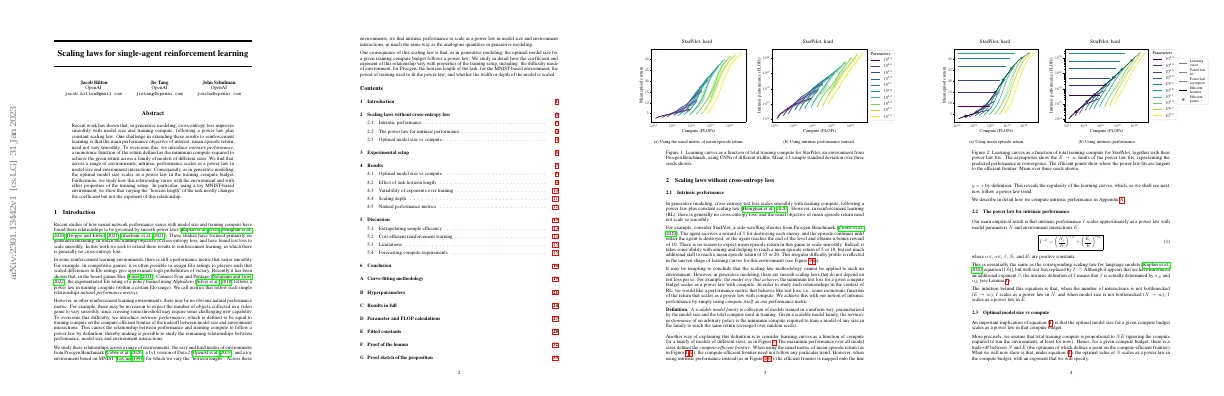
• Closeness of power law fit to learning curves shown in Figure 2 and Appendix C
• Primary determinant of exponents is domain
• Within MNIST, increasing horizon lowers exponent
• Within Procgen, easy and hard modes have similar exponents
• Difficulty mode does not affect scaling exponents

Effect of task horizon length

• MNIST experiments were used to artificially alter the “horizon length” of the task by setting the GAE credit assignment parameter λ to 1 and varying the GAE discount rate γ.
• Proposition 1 states that the covariance matrix of the policy gradient is approximately for some symmetric positive semi-definite matrices Σ θ and Π θ that do not depend on h.
• Gradient variance is an affine function of h (i.e., a linear function with an intercept).
• The number of environment interactions required should be an affine function of h.
• Results show that the number of interactions closely follows an affine function of the horizon length.
• Increasing the horizon length shifts the optimal model size vs compute curve to the right.
• Task horizon length is influenced by how long rewards are delayed for relative to the actions the agent is currently learning.

Variability of exponents over training

• Power law for intrinsic performance holds across environments and model sizes
• Scaling constants vary over the course of training
• Fitted power law to three different periods of training
• Early and middle periods of training have significantly lower scaling constants
• Measurement of scaling constants is an extrapolation if learning curves don’t reach compute-efficient frontier
• Exclude first 1/64 of training for other environments

Scaling depth

• Experiments involved scaling width and depth of networks
• Power law for intrinsic performance held, but with more noise
• Fitted values of α N and α E for depth-scaling experiments similar to width-scaling experiments
• Optimal model size for given compute budget smaller for depth-scaling experiments
• Optimal model size vs compute scaling laws more similar if measured using FLOPs per forward pass

Natural performance metrics

• Natural performance metrics can be found in some environments
• CoinRun: fail-to-success ratio is a natural performance metric
• Dota 2: TrueSkill rating system is a natural performance metric
• Intrinsic performance and natural performance metric fit closely, except for Dota 2 at higher levels

Discussion

Extrapolating sample efficiency

• We can use a power law to extrapolate sample efficiency to unseen model sizes and environment interactions.
• We can compare the extrapolated infinite-width limit to human sample efficiency.
• On StarPilot, humans are around 10,000 times more sample efficient than the extrapolated infinitely-wide model.

Cost-efficient reinforcement learning

• Sample efficiency is the primary metric of algorithmic progress in reinforcement learning.
• The cost of running the environment and the algorithm can both be taken into account.
• It is usually inefficient to use a model that is much cheaper to run than the environment when training from scratch.

Limitations

• Not separate training runs for each compute budget
• Variability of exponents over training
• Not carefully optimized aspect ratios
• High-variance learning curves

Forecasting compute requirements

• Scaling exponents for reinforcement learning lie in a similar range to generative modeling
• Scaling coefficients for reinforcement learning vary by multiple orders of magnitude
• Arithmetic intensity may confound scaling coefficients
• Sample efficiency is an affine function of the task horizon length
• Training data requirements are a sum of two components
• Continuing to increase the horizon length will eventually lead to a proportional increase in the compute budget
• Measuring scaling exponents precisely is challenging

Conclusion

• Extending scaling laws to single-agent reinforcement learning
• Notion of intrinsic performance
• Intrinsic performance scales as a power law in model size and environment interactions
• Optimal model size scales as a power law in the training compute budget
• Relationship affected by various properties of the training setup
• Implications for biological anchors framework for forecasting transformative artificial intelligence
• Computing intrinsic performance and fitting the power law constants require some care
• Intrinsic performance is the minimum compute required to train a model of any size
• Jointly fit the power law constants and a monotonic function
• Fit log (f ) rather than f
• Weight the data in proportion to 1 E
• Smooth learning curves
• Exclude data from early in training
• Greedy adaptive batch size algorithm
• Batch size schedule can be approximated by a power law
• Batch size schedule works well on different Procgen environments
• Batch size schedule works well on MNIST environment
• Tuning B min important for MNIST environment
• No batch size schedule used for Dota 2 experiments