Link to paper
The full paper is available here.
You can also find the paper on PapersWithCode here.
Abstract
- HMC is an algorithm to sample latent variables from Bayesian models
- PPLs allow users to focus on modeling instead of writing inference algorithms
- HMC can be difficult to use for some models, requiring tricks like reparameterization
- Marginalization can simplify models and improve sampling from hierarchical models
Paper Content
Introduction
- PPLs automate Bayesian reasoning
- User specifies probabilistic model and provides data
- PPLs have had tremendous impact in applied sciences
- PPLs vary in distributions and inference approach
- Focus on generative PPLs and programs that correspond to a graphical model
- Can reformulate model so some latent variables are generated after all observed variables
- Reducing number of variables for MCMC can lead to performance gains
- Automatically marginalize variables in user-specified probabilistic program for inference with HMC
Motivating examples
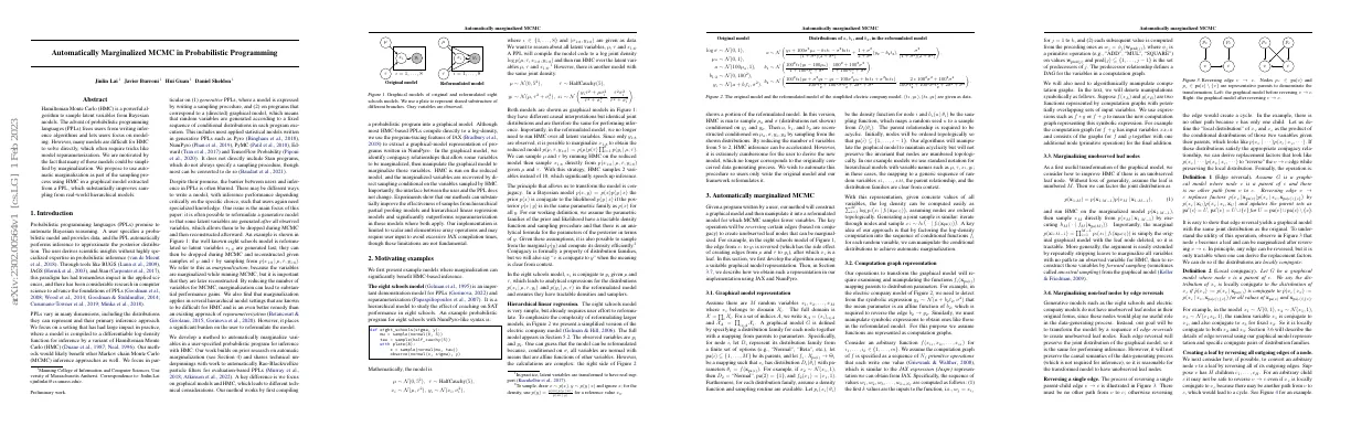
- Eight Schools model is an example of a hierarchical model to study the effect of coaching on SAT performance in eight schools
- The model is mathematically represented by µ ∼ N (0, 5 2 ), τ ∼ HalfCauchy(5)
- There is another model with the same joint density, but different causal interpretation
- HMC inference can be sped up by marginalizing x 1:8 and running HMC on the reduced model
- Conjugacy is a property of distribution families that allows for the transformation of the model
- In the eight schools model, x i is conjugate to y i given µ and τ
- Hierarchical linear regression is a more complex model that requires user effort to reformulate
Automatically marginalized mcmc
- Our method will construct a graphical model and manipulate it to reduce the number of variables.
- Certain edges will be reversed to create unobserved leaf nodes that can be marginalized.
- Algorithm is developed assuming a suitable graphical model representation.
Graphical model representation
- There are M random variables x 1 , x 2 , . . . , x M
- Each variable belongs to a domain X i
- A graphical model G is defined by specifying a distribution family for each node and a mapping from parents to parameters
- The parent relationship must be acyclic
- The log density can be computed easily
- Generating a joint sample is similar
- The approach allows for automatic marginalization
Computation graph representation
- Operations to transform graphical model require examining and manipulating functions.
- Functions are represented as computation graphs.
- Computation graphs are specified as a sequence of primitive operations.
- Manipulations of computation graphs are symbolically represented.
- Computation graph for a symbolic expression has input variables and consists of graphs for each expression plus one additional node.
Marginalizing unobserved leaf nodes
- HMC can be improved by deleting an unobserved leaf node
- Marginalizing all variables with no path to an observed variable can be done by repeatedly stripping leaves and running HMC on the marginalized model
Marginalizing non-leaf nodes by edge reversals
- Generative models do not have unobserved leaf nodes in their original forms
- Goal is to transform the model by a sequence of edge reversals to create unobserved leaf nodes
- Edge reversal preserves the joint distribution of the graphical model
- Local distribution of two variables is the product of their conditional distributions
- If distributions satisfy conjugacy relationship, replacement factors can be derived
- Reversing a single edge creates a leaf node that can be marginalized
- Reversing all outgoing edges of a node can convert it to a leaf
- MARGINALIZE function attempts to marginalize every node in reverse topological order
- RECOVER function augments a sample of non-marginalized variables with direct samples of marginalized variables
Conjugacy detection
- Detecting when x a is locally conjugate to x b uses patterns listed in Table 1
- AFFINE(u, v) means u can be written as u = pv + q for expressions p and q that do not contain v
- DEPENDENT(u, v) means there exists a path from v to u in the computation graph
- LINEAR(u, v) means u can be written as u = pv
Edge reversal details
- Algorithm 1 calls REVERSE operation to reverse an edge when conjugacy is detected
- Algorithm 2 shows portion of REVERSE algorithm for normal-normal conjugacy
- Operations like +, − and * are symbolic operations on computation graphs
- Algorithm implements Gaussian marginalization and conditioning formulas
- Line 5 extracts symbolic expressions for parameters of normal distributions
- Line 6 extracts expressions p and q such that µ c = px v + q
- Lines 7-13 compute symbolic expressions for parameters of marginal and conditional and write them to f c and f v
- Lines 15-16 update DAG to reflect new dependencies
Implementation
- Automatically marginalized HMC can be achieved by a pipeline of steps
- Steps include extracting a graphical model, calling a MARGINAL-IZE function, running HMC, and running Algorithm 2 for each HMC sample
Related work
- Conjugacy and marginalization are important topics in probabilistic programming
- Automatic Gibbs sampling can be improved using conjugacy
- Symbolic integrators can be used to perform marginalization for exact inference
- Graphical models can be used to identify patterns for efficient large scale models
- Autoconj proposes a term-graph rewriting system for marginalizing log joint density with conjugacy
- Delayed sampling uses automatic marginalization to improve inference
- Semi-symbolic inference expands the applicability of delayed sampling
- MCMC inference can be improved using HMC inference
- Stan programs specify a log-density and not a sampling procedure
- Reparameterization can be used in models where some variables are marginalizable
Experiments
- Evaluated performance of method on two classes of hierarchical models
- Used NumPyro’s no-U-turn sampler (NUTS)
- Approach was “HMC with marginalization” (HMC-M)
- Used 10,000 warm up samples to tune sampler, 100,000 samples for evaluation
- Evaluated performance via effective sample size (ESS) and time
Hierarchical partial pooling models
- Hierarchical partial pooling (HPP) model has a form that includes observed covariate and response values, local and global latent variables
- Some HPPs use conjugate distributions for local latent variables
- HMC struggles to sample small values of global latent variables due to a “funnel” relationship
- Marginalization eliminates the funnel and improves the quality of samples
- HPPs can be used for repeated binary trials
- Sampling global latent variables is difficult, but HMC-M achieves an ESS with similar magnitude to the number of samples
- HMC problem dimension is reduced, leading to faster running time and more than 100x ESS/s improvement
Hierarchical linear regression
- Hierarchy can be introduced in linear regression models.
- Examples are given to show how methods can improve inference.
- Variables can be marginalized from the HMC process.
Discussion
- Proposed a framework to automatically marginalize variables in graphical models
- Results show significant performance improvements in models with conjugacy
- Process can be automated to free users from cumbersome derivations and implementations
- Method is limited to graphical models, excludes some PPL features
- Current implementation is limited to scalar and elementwise array operations
- Future work includes supporting wider range of array operations and introducing automatic marginalization to higher order PPLs
A. proof of the correctness of definition 1
- Definition 1 is Edge Reversal
- Edge Reversal replaces factors and updates parent sets
- Proven that Edge Reversal yields same joint distribution as original
- No cycles formed during process
- No other paths from v to c
B. proof of the theorem 1
- Theorem 1 states that a node can be turned into a leaf by sorting its children and reversing the edges from the node to each child.
- The proof is done by induction.
- The three conditions of local conjugacy in Table 1 will not change after the reversal.
- The theorem is proven by showing that the three conditions hold for k = H.
F. slow compilation of jax
- JAX compilation time can be slow for some models
- Problem identified in marginalized hierarchical models
- JIT compilation time scales super-linear with respect to N for the marginalized model
- JIT compilation time for the gradient function of the marginalized model can be hundreds larger than that of the original model when N is large enough
- Marginalization creates a chain shaped computation graph which is difficult for JAX to work with