Link to paper

The full paper is available here.

You can also find the paper on PapersWithCode here.

Abstract

• Problem of learning a single neuron with ReLU activation under Gaussian input with square loss is revisited.
• Over-parameterization setting (student network has $n\ge 2$ neurons) is focused on.
• Global convergence of randomly initialized gradient descent with a $O\left(T^{-3}\right)$ rate is proven.
• $\Omega\left(T^{-3}\right)$ lower bound for randomly initialized gradient flow in the over-parameterization setting is presented.
• Over-parameterization can exponentially slow down the convergence rate.

Paper Content

Introduction

• Gradient descent (GD) is used to train deep neural networks
• Over-parameterization plays a key role in successful training
• Over-parameterization can slow down convergence of GD
• Two-layer ReLU networks with n neurons and input dimension d are studied
• Student network is trained to learn a ground truth teacher network
• Square loss is considered
• Teacher network consists of one single neuron
• Student network is initialized with a Gaussian distribution
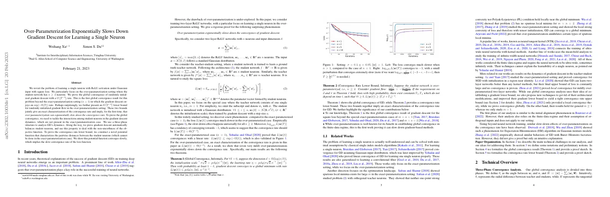
• Empirically, over-parameterization exponentially slows down convergence
• Theorem 1 shows global convergence of GD
• Theorem 2 provides a convergence rate lower bound
• Over-parameterization can slow down gradient-based methods

Related works

• Problem of learning a single neuron is well-understood
• Classical single index models algorithms can solve it
• GD can converge for learning a single neuron
• GD can converge for learning a convolutional filter
• Over-parameterization setting studied
• Optimization landscape studied
• GD can converge to global minimum with tensor initialization
• Over-parameterization can eliminate certain types of spurious local minima
• Neural tangent kernel connects training of ultra-wide neural networks with kernel methods
• Mean-field analysis studies training of infinite-width neural networks
• GD can learn two-layer networks better than kernel methods
• GD can converge globally

Technical overview

• Three-phase convergence analysis is divided into three phases
• θ i represents the radial difference between teacher and students, while H represents the tangential difference
• When initialization is small enough, in phase 1, θ i decreases while w i remains small
• In phase 2, θ i remains bounded while H decreases exponentially
• In phase 3, two properties are established: lower bound of gradient and regularity condition of student neurons
• Optimization landscape is different and harder to analyze when network is over-parameterized
• Loss function is not smooth when student neurons are close to 0
• GD implicitly regularizes student neurons and keeps them away from non-smooth regions near 0
• Gradient lower bound is improved from Ω(L(w)) to Ω(L 2/3 (w))
• Non-degeneracy condition is established to build lower bound of convergence rate

Preliminaries

• Bold-faced letters denote vectors
• [n] denotes {1, 2, . . . , n}
• θ(w, v) denotes the angle between two nonzero vectors w, v
• ∇ i denotes the gradient of the i th student neuron
• w(t) denotes the value of a variable at the t th iteration
• Expectation taken w.r.t the standard Gaussian is abbreviated
• Length of the projection of w i onto v is defined
• Closed form expressions of L(w) and ∇L(w) can be obtained
• Proof sketch for Theorem 1 provided

Initialization

• Initialization of w i (0) has high probability
• Norms of w i (0) have upper and lower bounds
• θ i will fall in the interval [ π 3 , 2π 3 ] initially

Phase 1

• Theorem 4 states that there are upper and lower bounds for w i
• Gradient norm is used to bound the dynamics of θ i
• θ i is small at the end of Phase 1
• Projections of student neurons on teacher neuron are balanced
• Proving upper bound of w i is straightforward
• Proving lower bound of w i is more difficult due to small perturbation term
• θ i remains small in second interval of Phase 1
• Increases of h i in second interval are balanced

Phase 2

• Phase 2 starts at time T1 + 1 and ends at time T2
• Theorem 5 states that projections hi remain balanced in Phase 2
• Equation 11 shows that hi remain balanced, 12 bounds the dynamics of H(t), 13 gives upper and lower bounds for hi, and 14 shows that θi remains upper bounded by a small term 2 in Phase 2
• Gradient (3) has the property that max i θi ≤ 2 and max i wi = O(v/n)
• H(t) exponentially decreases and gives upper and lower bounds
• Dynamics of cos θi is calculated and a potential function V(t) is defined
• Upper bound for V yields the final upper bound for θi

Phase 3

• Theorem 6 states that the desired 1/T3 convergence rate can be achieved.
• Prove a gradient lower bound ∇L(w) ≥ poly(n-1, v-1)L2/3(w).
• Prove that the loss function is smooth and Lipschitz on the gradient trajectory.
• Improved version of Theorem 3 in Zhou et al. [2021].
• Pick a global minimum w1, w2, …, wn and lower bound the projection of gradient on the direction wi - wi.
• Upper bound wi - w*i.
• Gradient lower bound scales with L2/3.
• Show that GD implicitly regularizes wi.
• Improved gradient lower bound is crucial for bounding the movement of student neurons.
• Convergence rate L(w(T)) ∼ 1/T2.

Main theorem

• Theorem 1 is formally stated and proven
• Parameters in Theorem 4, 5, 6 are assigned values (listed in Appendix E.2)
• Combining the initialization condition (Lemma 3) and three phases of analysis (Theorem 4, 5, 6) proves Theorem 9
• Corner case of w i = 0 is excluded in the analysis (discussed in Appendix E.3)

Proof overview: convergence rate lower bound

• Gradient flow (gradient descent with infinitesimal step size) is considered
• Other settings (network architecture, initialization scheme, etc.) are kept unchanged
• Over-parameterization causes a significant change of the convergence rate
• Several toy cases are investigated to understand why

Case study

• w 1 and w 2 are reflection symmetric with respect to v
• gradient descent preserves the symmetry of w 1 and w 2
• λ 1 and λ 2 converge to 0 with rate λ 2 (t) ∼ t −1
• all student neurons are parallel with the teacher neuron: convergence rate is linear
• all student neurons are equal: training process is equivalent to learning one teacher neuron with one student neuron, step size multiplied by a factor of n

Non-degeneracy

• Theorem 9 gives a worst case optimal convergence rate.
• Theorem 12 gives an average case lower bound for the convergence rate.
• Theorem 12 requires random initialization to be non-degenerate.
• Theorem 12 depends on 1/κ-2 max (0).

Proof sketch

• Theorem 12 is proven by considering a potential function Z(t)
• The potential function explains why the convergence rate is different for n = 1 and n ≥ 2
• The potential function also explains why the convergence rates in two counter-examples are linear
• Several technical properties of the gradient flow trajectory are needed
• Lower bounding κ max is the most non-trivial step
• Lemma 15 states that when vectors are too close in direction, gradient flow will automatically separate them
• Remark 16 states that in toy case 3, all z i ’s remain parallel and will not be separated
• Closed form expressions for L and ∇L are presented
• Global convergence is shown in Theorem 4

C global convergence: phase 2

• Theorem 5 states that if the initial condition in Lemma 3 holds, then (40), (41), (42) and (43) hold.
• Proof of (40) involves computing a bound using (27) and (23).
• Proof of (41) involves computing a bound using (35) and (37).
• Proof of (42) involves computing a bound using (35) and (46).
• Proof of (43) involves computing a bound using (29), (31) and (34).
• Lemma 17 states that at the start of Phase 3, the conditions (40), (41), (42) and (43) in Theorem 5 are satisfied.
• Proof of Lemma 17 involves computing a bound using (34) and (37).

D.2 proofs for gradient lower bound

• Lemma 8 introduces the idea of residual decomposition
• Lemma 18 provides a bound of θi
• Lemma 19 provides a bound of r
• Theorem 7 states that if certain conditions are met, then the global minimum can be found

D.3 handling non-smoothness

• Set 2 = O(n-14)
• Set 84.5 = O(n-14)
• Set nη = O(n-14)
• Lemma 21 ensures smoothness of L when student neurons are regularized
• Lemma 22 ensures student neurons won’t move too far in phase 3
• Theorem 6 sets parameters according to Theorem 4 and Theorem 5
• Theorem 7 bounds decrease of loss at time t
• Theorem 8 ensures properties hold with probability at least 1-δ

E.3 non-degeneracy of student neurons

• Technical issue: student neuron w i can be degenerate and w i = 0, making loss function L(w) not differentiable
• Proof shows student neurons are always non-degenerate
• Student neuron’s norm w i is always lower-bounded in all three phases of analysis
• Corollary describing non-degeneracy of student neurons
• Assumption on initialization condition necessary, otherwise counter-examples exist
• Technical preparations for proving Theorem 12
• Gradient flow version of Theorem 6 and Corollary 23
• Lemma 27: given non-degenerate initialization, at least one student neuron z i (t) = 0
• Lemma 28: given non-degenerate initialization, at least one of two conditions must hold
• Lemma 29: given non-degenerate initialization, Z(t) ≥ Ω(κ max (0) max i∈ [n] z i (t) )
• Corollary 30: given conditions, Z(t) > 0
• Lemma 31: given conditions, ∂ ∂t Z(t) ≥ −O(n 2 v θ 2 max (t))