Link to paper

The full paper is available here.

You can also find the paper on PapersWithCode here.

Abstract

• Transfer learning is the dominant paradigm of machine learning.
• Pre-trained models can be fine-tuned for downstream tasks with fewer labelled examples.
• Modular deep learning is a promising solution to challenges of positive transfer and systematic generalisation.
• Modular architectures provide a unified view of research that evolved independently.
• Modularity can be used for scaling language models, causal inference, programme induction, and planning in reinforcement learning.
• Modularity has been successfully deployed in cross-lingual and cross-modal knowledge transfer.

Paper Content

Introduction and motivation

• Transfer learning is a popular machine learning technology
• Pre-training a model on raw data and fine-tuning it for new tasks is successful but has limitations
• Modularity in artificial and biological systems is beneficial for evolvability, adaptability, and resilience
• Vanilla neural networks can learn a modular pattern
• Modular neural architectures have advantages such as positive transfer, compositionality, and parameter efficiency
• Modules can be implemented in different ways
• Routing functions control the flow of information to the modules
• Aggregation strategies are used when multiple modules are selected
• Modules can be trained in different ways
• Modularity is beneficial in transfer learning, causal inference, and programme simulation
• Modular deep learning can be used in natural language processing, computer vision, and speech processing

Modular deep learning

• Focuses on modular deep learning models composed of modules
• Modules are autonomous computation functions referred to as adapters, options, or experts
• Distinguished from routing function which controls information flow
• Aggregation function aggregates outputs
• Modules can be combined with fully shared parameters
• Taxonomy of four dimensions of variation: computation, routing, aggregation, and training

Taxonomy

• A module may consist of any component of a neural architecture
• Routing function is either fixed or learned
• Aggregation function is either deterministic or learnable
• Modules can be trained jointly or post-hoc

Notation

• Neural network decomposed into graph of sub-functions
• Graph is a linear chain
• Sub-functions refer to model’s layers with unique indexed parameters
• Parameters can be further decomposed recursively
• Modules can be modified by parameter composition, concatenation, or feeding output of one function into another
• Routing function returns score for each module conditioned on data or metadata
• Routing function can be hard, soft, or unnormalised score vector
• Output of each module combined through aggregation function
• Aggregation function can be deterministic or learnable neural network

Computation function

• Computation function determines module design
• Different module architectures proposed
• Most often modules integrated into base architecture with shared parameters
• Three core methods to merge single module with ([φ, x])

Routing function

• Fixed routing is a method of generating modular parameters conditioned on metadata.
• Fixed routing is applicable to function composition.
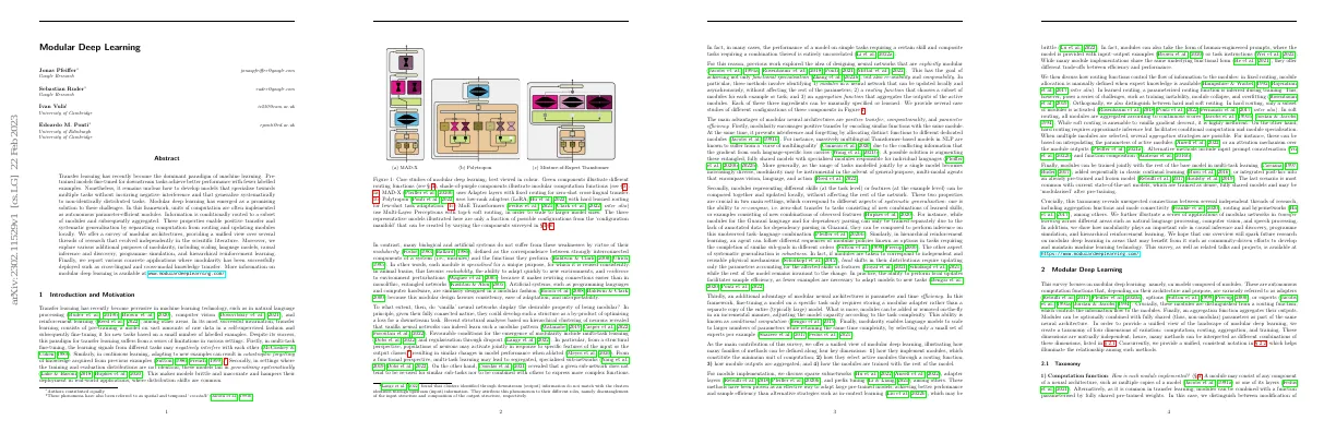
• There are three methods of instantiating modules: parameter composition, input composition, and function composition.
• Examples of the three computation functions are provided in Figure 2 and discussed in Table 3.

Parameter composition

• Parameter composition methods augment a base model with weights and module parameters to make the model more parameter-efficient.
• Sparsity is a common inductive bias based on the assumptions that only a small number of parameters are relevant for a particular task and that similar tasks share similar sub-networks.
• Pruning is the most widespread method to induce sparsity, which can be interpreted as the application of a binary mask.
• Iterative pruning is carried out over multiple stages and often retains or surpasses the performance of the original dense model.
• Winning tickets have been shown to exist in RL, NLP, and computer vision.
• Pruning based on first-order (gradient-based) information better captures the task-specific relevance of each weight.
• Sparsification techniques can be employed for adaptation, such as Sparse Fine-Tuning and Diff pruning.
• Low-rank modules can also be used to save space and time.
• Parameter composition methods are very parameter-efficient and often require updating less than 0.5% of a model’s parameters.

Input composition

• Input composition methods add a parameter vector to a function’s input.
• Common strategy is to add the parameter vector to the model’s first layer.
• Task-specific text prompt is converted to natural language and corresponds to modular parameters.
• Continuous prompt vector can be learned directly.
• Module vectors can be learned for each layer of the model.

Function composition

• Parameter composition deals with individual weights
• Input composition methods act on a function’s input
• Function composition methods add new task-specific sub-functions
• Parameter sharing models in multi-task learning consist of shared layers
• Multi-task architecture can be obtained by tying sets of parameters between models
• Cross-stitch unit linearly combines inputs at every layer
• Sluice networks extend cross-stitch units to multiple modules per layer
• Adapter layers are an alternative to parameter sharing
• Adapter layers are composed with a pre-trained model
• Adapter layers are modality-specific
• Adapter layers can be routed sequentially or in parallel

Hypernetworks

• Hypernetworks are a third kind of routing with unnormalised routing scores.
• Parameters for a task are generated by a linear function.
• Task embedding is the output of a task-level routing function with unnormalised scores.
• Generator is a matrix of module parameters stacked column-wise.
• Parameters are a linear combination of the columns of the linear generator.
• Hypernetworks learn both sets of parameters jointly.

Unifying parameter, input, and function composition

• All modular computation functions can be reduced to function composition.
• Function composition methods use a weighted addition, while parameter and function composition use an unweighted addition.
• Different methods have different trade-offs in terms of capacity, memory footprint, and performance.
• Routing, aggregation, and training settings for the modules are discussed in the following sections.

Routing function

• A decision-making process is required to determine which modules are active in a modular neural architecture.
• This process is implemented through a routing function.
• When metadata is available, the routing decision can be made a priori.
• When no prior information is available, the routing function needs to be learned.
• Learning-to-route can be split into hard routing and soft routing.

Fixed routing

• Making routing decisions based on metadata is referred to as fixed routing
• Fixed routing simplifies the routing function to selecting a subset of modules
• An example of fixed routing is when all parameters, except the final classification layer, are shared among all tasks
• Methods that adapt pre-trained models towards individual tasks also route representations through a newly introduced module
• Fixed routing can select separate language and task components
• Fixed routing can also be based on other metadata such as language, domain, or modality information

Learned routing

• Routing function can be implemented as a learnable neural network
• Learning the routing function implies that the specialisation of each module is unknown
• Training instability, module collapse, and overfitting are challenges
• Challenges are caused by need to balance between exploration and exploitation and sharing modules across examples or tasks
• Training instability can be mitigated by curriculum learning or training the router parameters with a different learning rate
• Module collapse can be avoided by -greedy routing, auxiliary losses, or intrinsic rewards
• Overfitting can be avoided by routing conditioned on metadata or favouring combinatorial behaviour of modules
• Hard routing can be learned via reinforcement learning, evolutionary algorithms, or stochastic re-parameterisation
• Soft routing uses a mixture of experts
• Token-level routing uses top-k selection to load balance computation

Level of routing

• Routing can be done globally, per layer, or hierarchically.
• Allowing for different decisions per layer is more challenging as the space of potential architectures grows exponentially.
• Routing scores are sometimes used to select a subset of modules and to aggregate their outputs.

Aggregation function

• Routing and aggregation of modules are performed simultaneously
• Strategies for aggregating functions are similar to the taxonomy discussed for computation functions
• Aggregation of modular components can be realised on the parameter level
• Output level aggregation is also discussed

Parameter aggregation

• Interpolating module weights can have catastrophic consequences
• Linear mode connectivity suggests that interpolation between multiple models is possible under certain conditions
• Mode paths are not usually linear
• Linear mode connectivity is linked to the Lottery Ticket Hypothesis
• Interpolation is connected to the flatness of the loss landscape
• Success of interpolation is connected to the optimiser used

Representation aggregation

• Representation aggregation is equivalent to parameter aggregation if the functions are linear.
• Representation aggregation does not work for non-linear functions.
• Representation aggregation involves interpolating the outputs of individual modules.
• Representation aggregation can be done by learning weights to interpolate hidden representations.
• Attention-based aggregation functions take into account the information content of the hidden representations.
• Top-k hard routing is more efficient for weighted averaging and attention-based aggregation.

Input aggregation

• Input aggregation is used to create adapters such as prompts or prefix tuning
• Hypernetworks can combine different embeddings in the input to the parameter generator
• Embeddings can represent the position of the generated parameters in the neural architecture

Function aggregation

• Aggregation can be achieved on the function level
• Different aggregation methods infer either a sequence or a tree structure
• Forward pass through multiple modules transforms hidden representations
• Pfeiffer et al. propose a two-stage setup for zero-shot cross-lingual transfer
• Stickland et al. perform function composition for multilingual multi-domain machine translation
• Neural Module Networks use a semantic parse to infer a graphical structure for module aggregation

Training setting

• All modules can be trained together for multi-task learning
• Modules can be introduced at different stages during continual learning
• Transfer learning involves adding modules post-hoc after pre-training

Joint multitask learning

• Joint multi-task learning has two main settings
• Task-specific parameterised components can be integrated into shared neural network architectures
• Alternative is to have a fully modular architecture, sharing only the parameters for learned routing
• Joint training can also be performed before post-hoc training

Continual learning

• Multi-task learning and continual learning aim to prevent catastrophic forgetting
• New layers can be added to the network to update new data while keeping the others untouched
• Progressive Networks scale the model capacity linearly with the number of tasks
• Separate experts can be trained for each task
• Subnetworks of the model can be identified and updated without affecting previously learned knowledge
• Supermasks can be used to extend to a vast number of tasks during continual learning

Parameter-efficient transfer learning

• Transfer learning is the dominating strategy for state-of-the-art results
• Models are pre-trained on large amounts of data and then fine-tuned on target tasks
• Parameter-efficient fine-tuning strategies exist
• Modularity can be achieved through parameter, input and function composition
• Hypernetworks can be used to generate parameters of modules
• All methods share the same functional form