Link to paper

The full paper is available here.

You can also find the paper on PapersWithCode here.

Abstract

• Markov state models are used to interpret molecular dynamics trajectories.
• Structurally distinct conformations are needed to understand the biomolecular process.
• Dihedral angles and interresidue distances are used as input coordinates.
• Contacts are used to define and select contact distances.
• Low-pass filtering and correlation-based characterization of states are used.
• States of the Markov model are discriminated by the features.

Paper Content

Introduction

• MSMs are popular for MD simulations
• Workflow to construct an MSM consists of: selection of suitable input coordinates, dimensionality reduction, clustering of low-dimensional data into metastable conformational states, and estimation of transition matrix
• Variational principle states that MSM producing slowest timescales represents best model
• Internal coordinates such as dihedral angles and interatomic distances are natural choice
• Interresidue distances number scales quadratically with number of residues
• Exclude irrelevant motions from analysis
• Correlation analysis termed MoSAIC block-diagonalizes correlation matrix
• Study on virtues and shortcomings of using contact distances or backbone dihedral angles
• Focusing on folding of villin headpiece (HP35)
• Employing 300 µs-long MD trajectory of HP35
• Comparing fraction of native contacts Q and sum Ψ over backbone dihedral angles ψi
• Contacts and dihedrals appear to monitor overall structural evolution of HP35
• Simulation data and intermediate results available on Github page

Feature selection

• Conducted a 300 µs-long MD simulation of HP35
• Used Amber ff99SB*-ILDN force-field and TIP3P water model
• 1.5 × 10^6 data points collected

Definition of contacts

• Conditions for contact established (distance cutoff)
• Choice of molecular structures (single crystal structure or MD structures)
• Definition of distance between residues (Cα-atoms or closest heavy atoms)
• Contact established if distance between closest non-hydrogen atoms is < 4.5 Å
• Residues must be more than 3 residues apart
• Contact must be populated > 30% of simulation time
• 42 native contacts found in MD trajectory
• Distance cutoff based on studies of distance distribution of proteins
• Exclude (n, n+3) contacts
• Fraction of native contacts highly correlated with RMSD of folding trajectory
• Exclude non-native contacts that are typically infrequent and short-lived
• Different choice of native contacts than crystal structure
• Appropriate calculation of contact distance crucial for modeling
• Exclude atom pairs that don’t meet population cutoff of 0.3

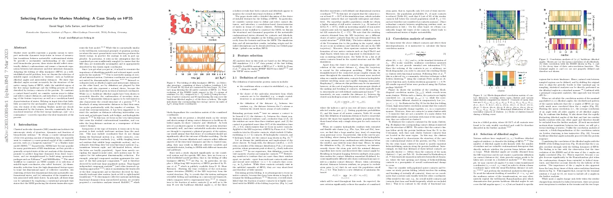
Correlation analysis of contacts

• Calculated linear correlation matrix to characterize contacts and detect interdependencies
• Blocked-diagonalized correlation matrix to associate blocks/clusters with functional motions
• Seven main clusters with high intracluster correlation and low correlation between different clusters
• Clusters follow protein backbone from N- to C-terminus
• Cluster 8 mostly represents helix-stabilizing contacts with shorter lifetimes than other clusters

Selection of dihedral angles

• Number of dihedral angles scales linearly with number of residues
• Dihedral angles indicate whether protein forms helices, sheets or loops
• Convert angles to sine/cosine-transformed coordinates
• Ramachandran plot shows protein backbone dihedral angles are limited to specific regions
• Correlation matrix of dihedral angles shows ψ angles are more correlated than φ angles
• ψ angles correlate strongly with folding dynamics of HP35

Construction of metastable states

• Employed Gaussian low-pass filter to eliminate high-frequent fluctuation of feature trajectory
• Used density-based clustering to generate microstates
• Used most probable path algorithm to lump microstates into macrostates
• Used projection method of Hummer and Szabo to construct transition matrix of metastable states

Dimensionality reduction

• PCA is a linear transformation that removes linear correlations among variables
• First PCs account for largest correlation of data set
• Aim to obtain low-dimensional representation by truncating number of PCs
• First 5 PCs explain 80% of total correlation
• First PC mostly reflects fraction of native contacts

Clustering

• Used robust density-based clustering to compute local free energy estimate for every frame of trajectory
• Reordered structures from low to high free energy to identify minima of free energy landscape
• Iteratively increased energy threshold to assign structures to same cluster until clusters meet at energy barriers
• Used hypersphere of radius 0.124 for contact distances and 0.072 for dihedral angles
• Used MPP algorithm to construct small number of macrostates
• Calculated transition matrix of microstates using lag time of 10 ns
• Self-transition probability of state lower than metastability criterion Qmin, state lumped with state to which transition probability is highest
• Repeated procedure for increasing Qmin to construct dendrogram showing topology and hierarchical structure of free energy landscape
• Obtained 12 metastable states for both contacts and dihedral angles

Structural characterization of states

• Obtaining a useful state model requires structurally well-defined and long-lived or metastable states.
• Contact distances and dihedral angles are used to characterize the states.
• The states are ordered by decreasing fraction of native contacts.
• The first three states are structurally well-defined native-like states.
• The unfolded basin mainly consists of states 9 to 12, which show different degrees of disorder.
• The MoSAIC clusters provide a concise characterization of the structure of the metastable states.
• 6 contacts or 10 dihedrals are sufficient to discriminate all metastable states with high accuracy.

Dynamical properties of states

• Calculate transition matrix to assess dynamical properties of states
• Diagonalize transition matrix to obtain eigenvalues and implied timescales
• Implied timescales should be constant for Markovian dynamics
• Probabilities reflect hydrophobic collapse, time in unfolded basin, and overall folding process
• Implied timescales level off for lag times of 10 ns
• Slowest timescale for contacts is 1.2 µs, for dihedrals is 0.7 µs
• Folding time defined as waiting time for transition from unfolded to native state
• MSM reproduces broad MD folding-time distributions
• Gaussian filtering improves implied timescales and structural characterization

Results on the folding of hp35

Ground truth observations

• MD simulation results include RMSD, native contacts, and sum of backbone dihedral angles
• Upper and lower thresholds of 2Å and 6Å for folded and unfolded conformations
• Free energy profile consists of two states, native and unfolded
• Transition path time is shorter than folding time
• Correlation between 1-Q and RMSD
• Sharp minimum for native state and shallow minimum for unfolded state in free energy profile
• Cooperative behavior of native contacts and dihedral angles
• Multiple folding pathways indicated by preferred but not mandatory cluster formation order
• Contact clusters and dihedral angles too coarse grained to accurately reproduce dynamics of system

Kinetic network and folding pathways

• Constructed MSMs of HP35 found 12 metastable states with well-defined structures

Discussion

Feature selection: contacts vs. dihedrals

• Model problem of ultrafast folding of HP35 studied
• Dihedral angles used as features to construct MSM
• Dihedral angles require appropriate treatment and exclusion of uncorrelated motion
• Maximal-gap shifted (φ, ψ) dihedral angles used
• Dihedral angles report on local secondary structure
• Contact distances require selection and appropriate calculation
• Correlation analysis identifies seven clusters of contacts
• Contacts key to folding process, give better Markovian model than dihedrals

Msm workflow: what matters?

• Selection of features is important
• PCA used to explain majority of correlation
• Robust density-based clustering used to construct microstates
• Gaussian low-pass filtering used to reduce spurious transitions
• Dendrograms used to reveal hierarchical structure of free energy landscape

Concluding remarks

• Aim to construct structurally well-defined metastable states to understand biomolecular process
• Use correlation analysis to identify appropriate features
• Quality of state partitioning can be assessed by MPP dendrogram
• Dynamical corrections can improve Markovianity of MSM
• Check if resulting metastable states are structurally well characterized
• Decision tree-based machine learning to identify essential coordinates
• MSMs correctly reproduce slow timescales of process
• Kinetic networks and state trajectories obtained from contacts and dihedrals
• Preselection of backbone dihedral angles
• Structural characterization of metastable states
• Cooperativity of input features during folding events
• Most probable folding pathways identified by MSMPathfinder