Link to paper

The full paper is available here.

You can also find the paper on PapersWithCode here.

Abstract

• Exogenous state variables and rewards can slow reinforcement learning.
• Reward function decomposes additively into endogenous and exogenous components.
• Decomposition of state space into exogenous and endogenous state spaces must be discovered.
• Algorithms introduced to discover exogenous and endogenous subspaces of state space.
• Experiments show that these methods produce speedups in reinforcement learning.

Paper Content

Introduction

• Actions of an agent have limited effect on environment
• Wireless cellular network has parameters that must be dynamically controlled
• Formulated as a Markov Decision Process (MDP)
• Reward function is negative of number of users with low bandwidth
• Reward heavily influenced by exogenous factors
• Stochasticity can confuse reinforcement learning algorithms
• Need many trials to average away exogenous components
• Learning rate needs to be small
• Number of Monte Carlo trials required to estimate gradient grows large
• Analyze setting and develop algorithms to detect and remove effects of exogenous state variables
• Accelerates reinforcement learning (RL)

Mdps with exogenous states and rewards

• Study of discrete time stationary MDPs with stochastic rewards and transitions
• State and action spaces can be discrete or continuous
• State space S, action space A, reward distribution R, transition function P, starting state distribution P0, discount factor γ
• For all (s, a) in S x A, R(s, a) has expected value m(s, a) and finite variance σ2(s, a)
• State space S takes form S = x d i=1 S i
• State s can be written as d-tuple of values of state variables s = (s1, …, sd)
• Random vector for state at time t is S t = x d i=i S t,i
• Random variable for action at time t is A t
• Random variable for reward at time t is R t
• State variables can be decomposed into endogenous and exogenous sets E and X
• Vector space of m x n matrices over R
• Linear decomposition of S into endo/exo parts E and X via W
• Direct Sum of vector spaces A and B
• Vector subspace of vector space B
• Orthogonal complement of subspace A of vector space S
• Dimension of vector subspace A
• Identity matrix of size n, Matrix of zeros of size m x n
• Matrix that defines the linear exogenous subspace
• Trace of matrix A, Transpose of A, Determinant of A
• Euclidean norm of vector u
• Covariance matrix of A, Cross-covariance matrix of A, B
• Gaussian distribution with mean µ and variance σ2

Exogenous state variables

• Exogeneity is a causal concept: a variable is exogenous if it is impossible for our actions to affect its value
• Formalized in terms of Pearl’s do-calculus
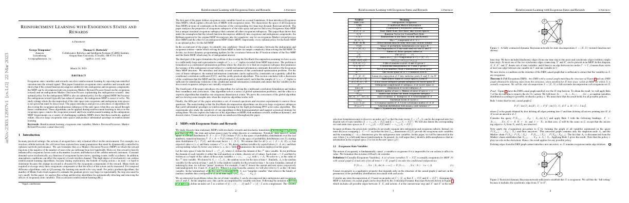
• A DBN with a certain structure is sufficient to ensure that the variables in X are exogenous
• Multiple exo/endo decompositions are possible for an MDP with exogenous state variables
• Not every subset of exogenous state variables can yield a valid exo/endo decomposition
• Interested in the exo/endo decomposition where the exo set X is as large as possible
• Maximal exo/endo decomposition is unique and contains all exogenous state variables
• Statistically exogenous variables can be inferred from data, but not necessarily causally exogenous

Additive reward decomposition

• Reinforcement learning can be accelerated when reward function can be decomposed into two functions
• One function depends on exogenous variables, the other depends on both exogenous and endogenous variables
• Mean and variance of exogenous and endogenous reward distributions can be calculated
• Bellman optimality equation can be decomposed into two separate equations
• Optimal policy for the endo-MDP is an optimal policy for the full exogenous state MDP
• McGregor et al. (2017) show how to remove known exogenous state variables to accelerate Model Free Monte Carlo algorithm

Variance analysis of the exo/endo decomposition

• Reinforcement learning on the endogenous MDP can be more efficient than on the original MDP
• Estimating the value of a fixed policy in a given start state via Monte Carlo trials of length H
• Sample complexity of estimating V π (s 0 ; H) on the full MDP compared to the sample complexity of estimating V π end (s 0 ; H) on the Endogenous MDP
• Define B π (s 0 ; H) to be a random variable for the H-step cumulative discounted return
• Theorem 5 states that the sample size bound using the endogenous MDP will be less than the required sample size using the full MDP
• Variance and covariance of the H-step returns need to be computed
• Algorithm 1 for discovering the exogenous variables of an MDP from data collected during exploration
• Exogenous state discovery problem formulated as finding a set of variables that minimizes the residuals of the fitted exogenous reward function
• Two variations of the optimization formulation
• Most general formulation in which the exo-endo decomposition is defined by a diffeomorphism
• Practical special case in which the exogenous and endogenous spaces are defined by a linear mapping

Variable selection formulation

• Variable selection formulation aims to find two disjoint sets of state variables
• Squared error of exogenous reward regression is minimized
• Conditional mutual information constraints are used to enforce structure
• Problem is broken into two subproblems
• Hierarchical formulation is a simpler proxy for the coupled formulation

Continuous formulation

• Continuous formulation assumes state space conditions
• Mapping should preserve probability densities
• Diffeomorphisms are a natural choice
• Diffeomorphisms do not lose information
• Probability density of transformation can be written analytically
• Mutual information and conditional independence are preserved
• Formulation jointly optimizes diffeomorphic state transformation and exogenous reward function
• Relaxed definition of diffeomorphism (L-diffeomorphism) allows for mappings that are bijective and continuously differentiable almost everywhere

Linear formulation

• Introduce a tractable formulation for continuous diffeomorphisms
• Consider the general linear group GL(d, R) of invertible linear transformations in vector space R d
• Define a linear mapping ξ exo from the full state space to the exogenous state space
• Define the endogenous state space as the orthogonal complement of the exogenous state space
• Represent the state-space decomposition defined by W = (W exo , W end )
• Impose the requirement that the columns of W exo consist of orthonormal vectors
• Estimate the expectations required in the optimization formulations from sample transitions
• Adopt linear regression for the exogenous reward regression problem
• Replace conditional mutual information with the conditional correlation coefficient (CCC)
• Express the coupled formulation of the exogenous subspace discovery problem for the full setting
• Express the linear hierarchical formulation for the full case

Conditions establishing sound inference

• MDPs with finite, discrete state and action spaces can be used to find valid exo/endo decompositions
• Exploration policy must be fully randomized to visit all states and execute all possible actions
• Admissible MDPs must have all states reachable from the start state and all policies must reach a terminal state in a finite number of steps
• Episodic MDPs must reset to the start state after reaching a terminal state
• Ergodic MDPs must have all states reachable from each other in a finite number of steps
• Conditional mutual information must be zero for a valid exo/endo decomposition
• Faithfulness assumption must be made to infer the structure of a causal graph from observational data
• PPO must be initialized to a fully-randomized policy to guarantee valid exogenous sets

Algorithms for decomposing an mdp into exogenous and endogenous components

• GRDS algorithm is based on linear hierarchical formulation of Equation (22)
• SRAS algorithm starts with d exo := 0 and adds one column at a time
• GRDS algorithm solves inner objective by iterating from d exo := d down to zero
• GRDS algorithm minimizes CCC and halts when it finds W exo with CCC <
• GRDS algorithm solves optimization problem on Stiefel manifold

Analysis of the global rank-descending scheme

• Assume linear regression is used to fit the exo reward function
• Directly analyzing Algorithm 2 is difficult due to estimation errors, approximations, and using CCC as a proxy for conditional independence
• Oracle-GRDS algorithm returns a matrix W exo that forms a valid exo/endo decomposition of the full form with maximal dimension
• Unique maximal subspace X max is unique and all other exogenous subspaces X must be contained within X max
• GRDS departs from the oracle version in three ways: CCC in place of CMI, parameter , and finite training sample
• Stepwise Rank Ascending Scheme (SRAS) constructs W exo incrementally by solving a sequence of small manifold optimization problems
• SRAS maintains current partial solution W exo, temporary matrix W temp, set of candidate column vectors C x, and orthonormal basis N for the null space of C x
• SRAS computes new candidate vector ŵ by solving a simplified CCC minimization problem on the Stiefel manifold
• SRAS checks if CCC is less than parameter , computes E matrix, and checks if CCC f ull is less than
• Not all subsets of the maximal exogenous subspace are valid exogenous subspaces, so SRAS does not terminate when adding a candidate vector to W exo causes the full constraint to be violated